In this tutorial, we’ll cover the following:
How to select climate datasets from the CMIP6 archive
Loading CMIP6 data stored in the Zarr format
Calculate climate indices for extreme weather forecasts
# !mamba uninstall -y odc-loader
# !mamba install -y cartopy obstore 'zarr>=3' 'python=3.11'
| import cartopy.crs as ccrs
import dask.diagnostics
import matplotlib.pyplot as plt
import obstore
import obstore.auth.planetary_computer
import pandas as pd
import planetary_computer
import pystac_client
import seaborn as sns
import tqdm
import xarray as xr
import xclim
import zarrPart 1: Getting cloud hosted CMIP6 data
The Coupled Model Intercomparison Project Phase 6 (CMIP6) dataset is a rich archive of modelling experiments carried out to predict the climate change impacts. The datasets are stored using the Zarr format, and we’ll go over how to access it.
Note: This section was adapted from https://
Sources:
CMIP6 data hosted on Google Cloud - https://
console .cloud .google .com /marketplace /details /noaa -public /cmip6 Pangeo/ESGF Cloud Data Access tutorial - https://
pangeo -data .github .io /pangeo -cmip6 -cloud /accessing _data .html
First, let’s open a CSV containing the list of CMIP6 datasets available
df = pd.read_csv("https://cmip6.storage.googleapis.com/pangeo-cmip6.csv")
print(f"Number of rows: {len(df)}")
df.head()
Number of rows: 514818
Over 500,000 rows! Let’s filter it down to the variable and experiment we’re interested in, e.g. daily max near-surface air temperature.
For the variable_id, you can look it up given some keyword at
https://
For the experiment_id, download the spreadsheet from
cmip6
Another good place to find the right model runs is https://
Below, we’ll filter to CMIP6 experiments matching:
Daily Maximum Near-Surface Air Temperature [K] (variable_id:
tasmax)Alternatively, you can choose
prto get precipitation
Shared Socioeconomic Pathway 3 (experiment_id:
ssp370)Alternatively, you can also try
ssp585for the worst case scenario
df_tasmax = df.query("variable_id == 'tasmax' & experiment_id == 'ssp370'")
df_tasmaxThere’s 376 modelled scenarios for SSP3. Let’s just get the URL to the last one in the list for now.
print(df_tasmax.zstore.iloc[-1])gs://cmip6/CMIP6/ScenarioMIP/CMCC/CMCC-ESM2/ssp370/r1i1p1f1/day/tasmax/gn/v20210202/
Part 2: Reading from the remote Zarr store
In many cases, you’ll need to first connect to the cloud provider. The CMIP6 dataset allows anonymous access, but for some cases, you may need to authentication.
We’ll connect to the CMIP6 Zarr store on Google Cloud using
zarr.storage.ObjectStore:
gcs_store = obstore.store.from_url(
    url="gs://cmip6/CMIP6/ScenarioMIP/CMCC/CMCC-ESM2/ssp370/r1i1p1f1/day/tasmax/gn/v20210202/",
    skip_signature=True,
)
store = zarr.storage.ObjectStore(store=gcs_store, read_only=True)
Once the Zarr store connection is in place, we can open it into an xarray.Dataset like so.
ds = xr.open_zarr(store=store, consolidated=True, zarr_format=2)
ds
/srv/conda/envs/notebook/lib/python3.11/site-packages/xarray_sentinel/esa_safe.py:7: UserWarning: pkg_resources is deprecated as an API. See https://setuptools.pypa.io/en/latest/pkg_resources.html. The pkg_resources package is slated for removal as early as 2025-11-30. Refrain from using this package or pin to Setuptools<81.
import pkg_resources
Selecting time slices
Let’s say we want to calculate temperature changes between
2025 and 2050. We can access just the specific time points
needed using xr.Dataset.sel.
tasmax_2025jan = ds.tasmax.sel(time="2025-01-16").squeeze()
tasmax_2050dec = ds.tasmax.sel(time="2050-12-16").squeeze()
Temperature change would just be 2050 minus 2025.
tasmax_change = tasmax_2050dec - tasmax_2025janNote that up to this point, we have not actually downloaded any (big) data yet from the cloud. This is all working based on metadata only.
To bring the data from the cloud to your local computer, call .compute.
This will take a while depending on your connection speed.
tasmax_change = tasmax_change.compute()We can do a quick plot to show how maximum near-surface temperature is predicted to change between 2025-2050 (from one modelled experiment).
tasmax_change.plot.imshow()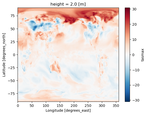
This temperature change is for the entire planet. Let’s zoom in over Vanuatu
projection = ccrs.epsg(code=3832)  # PDC Mercator
fig, ax = plt.subplots(nrows=1, ncols=1, subplot_kw=dict(projection=projection))
tasmax_change.sel(lon=slice(166, 170), lat=slice(-22, -11)).plot.imshow(
    ax=ax, transform=ccrs.PlateCarree()
)
ax.set_extent(extents=[166, 170, -22, -11], crs=ccrs.PlateCarree())
ax.coastlines()
<cartopy.mpl.feature_artist.FeatureArtist at 0x7f0e6fa48490>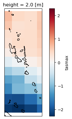
This CMIP6 output is very coarse, so there’s only 4x11=44 pixels covering Vanuatu. You could try to say that the northern regions is forecasted to experience higher daily maximum temperatures than the South in 2050 compared to 2025, but it’s best to get more data before jumping to these conclusions. Specifically:
Look at an ensemble of forecasts from different CMIP6 models
Potentially look at downscaled data that will show local patterns.
Part 2b: Getting downscaled climate data
For a small country like Vanuatu that is ~400km wide by ~800km long, it may be desirable to obtain higher spatial resolution projections. The original CMIP6 datasets have a coarse spatial resolution of 1 arc degree or more (>100 km).
There are groups that have taken these CMIP6 datasets and processed them using statistical downscaling + bias correction algorithms to produce higher spatial resolution outputs of 0.25 arc degrees (~25km) or so. Examples include:
Climate Impact Lab’s Global Downscaled Projections for Climate Impacts Research
NASA Earth Exchange Global Daily Downscaled Projection (NEX-GDDP-CMIP6)
Carbonplan’s CMIP6 downscaled products based on 4 different methods
References:
Gergel, D. R., Malevich, S. B., McCusker, K. E., Tenezakis, E., Delgado, M. T., Fish, M. A., and Kopp, R. E.: Global Downscaled Projections for Climate Impacts Research (GDPCIR): preserving quantile trends for modeling future climate impacts, Geosci. Model Dev., 17, 191–227, Gergel et al. (2024), 2024.
Thrasher, B., Wang, W., Michaelis, A., Melton, F., Lee, T., & Nemani, R. (2022). NASA Global Daily Downscaled Projections, CMIP6. Scientific Data, 9(1), 262. https://
doi .org /10 .1038 /s41597 -022 -01393-4
The examples below will use the CIL-GDPCIR-CC0 dataset hosted on Planetary Computer
catalog = pystac_client.Client.open(
    "https://planetarycomputer.microsoft.com/api/stac/v1/",
    modifier=planetary_computer.sign_inplace,
)
SSP_ID = "ssp585" # "historical", "ssp126", "ssp245", "ssp370", "ssp585"
search = catalog.search(
collections=["cil-gdpcir-cc0"], # add "cil-gdpcir-cc-by" for more models
query={"cmip6:experiment_id": {"eq": SSP_ID}},
)
ensemble = search.item_collection()
len(ensemble)3Let’s look at precipitation (pr).
Code based on:
# select this variable ID for all models in a collection
variable_id = "pr"  # or "tasmax"

datasets_by_model = []

for item in tqdm.tqdm(ensemble):
    asset = item.assets[variable_id]
    # print(asset.href, asset.extra_fields["xarray:open_kwargs"])

    credential_provider = (
        obstore.auth.planetary_computer.PlanetaryComputerCredentialProvider(
            url=asset.href, account_name="rhgeuwest"
        )
    )
    azure_store = obstore.store.from_url(
        url=asset.href, credential_provider=credential_provider
    )

    zarr_store = zarr.storage.ObjectStore(store=azure_store, read_only=True)
    datasets_by_model.append(xr.open_zarr(store=zarr_store, chunks={}))

all_datasets = xr.concat(
    datasets_by_model,
    dim=pd.Index([ds.attrs["source_id"] for ds in datasets_by_model], name="model"),
    combine_attrs="drop_conflicts",
)
100%|██████████| 3/3 [00:12<00:00, 4.12s/it]
all_datasetsWe now have a data cube consisting of 3 models, spanning a time range from 2015 to 2100. Let’s subset the data over Vanuatu.
ds_vanuatu = all_datasets.sel(lon=slice(166, 170), lat=slice(-22, -11))
ds_vanuatuPart 3: Compute climate indicators using xclim
The xclim library allows us to compute climate indicators based on
some statistic from raw climate values such as temperature or precipitation.
We’ll learn how to calculate a ‘drought’ indicator in this section. Specifically, compute maximum consecutive dry days with threshold of <1 mm/day.
da_cdd = xclim.indicators.atmos.maximum_consecutive_dry_days(
    ds=ds_vanuatu,
    thresh="1 mm/day",
)
da_cdd
/srv/conda/envs/notebook/lib/python3.11/site-packages/xclim/core/cfchecks.py:77: UserWarning: Variable does not have a `cell_methods` attribute.
_check_cell_methods(getattr(vardata, "cell_methods", None), data["cell_methods"])
/srv/conda/envs/notebook/lib/python3.11/site-packages/xclim/core/cfchecks.py:79: UserWarning: Variable does not have a `standard_name` attribute.
check_valid(vardata, "standard_name", data["standard_name"])
We have 3 models, over 86 timesteps (2015-2100), across 44x16 pixels over Vanuatu. Let’s compute this ‘drought’ indicator for one model and one year only.
with dask.diagnostics.ProgressBar():
    vu_cdd = da_cdd.isel(model=0, time=-1).compute()
[########################################] | 100% Completed | 15.33 ss
projection = ccrs.epsg(code=3832)  # PDC Mercator
fig, ax = plt.subplots(nrows=1, ncols=1, subplot_kw=dict(projection=projection))
vu_cdd.sel(lon=slice(166, 170), lat=slice(-22, -11)).plot.imshow(
    ax=ax, transform=ccrs.PlateCarree()
)
ax.set_extent(extents=[166, 170, -22, -11], crs=ccrs.PlateCarree())
ax.coastlines()
<cartopy.mpl.feature_artist.FeatureArtist at 0x7f0ded106a90>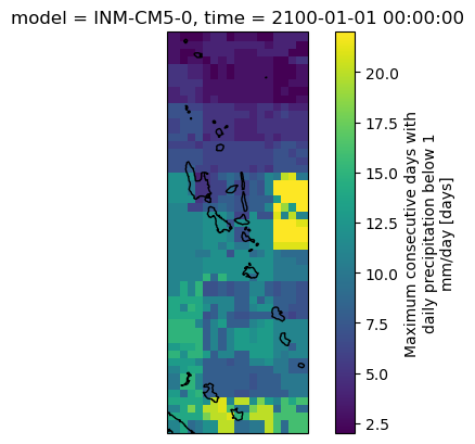
Let’s now compute this ‘drought’ indicator from 2025-2075, over an ensemble of three models. This will take about 5min to compute.
with dask.diagnostics.ProgressBar():
    vu_cdd = da_cdd.sel(time=slice("2025", "2075")).compute()
[########################################] | 100% Completed | 303.63 s
Over the 44x16 pixels over Vanuatu, we’ll get the maximum of all maximum
consecutive dry day (cdd) values, per model. The .max (highest) value is taken,
because we are interested in extreme values in terms of many dry days, but you
could also get the .median statistic or .min (lowest) statistic.
cdd_mean = vu_cdd.max(dim=("lat", "lon"))
cdd_meancdd_mean.plot.line(x="time")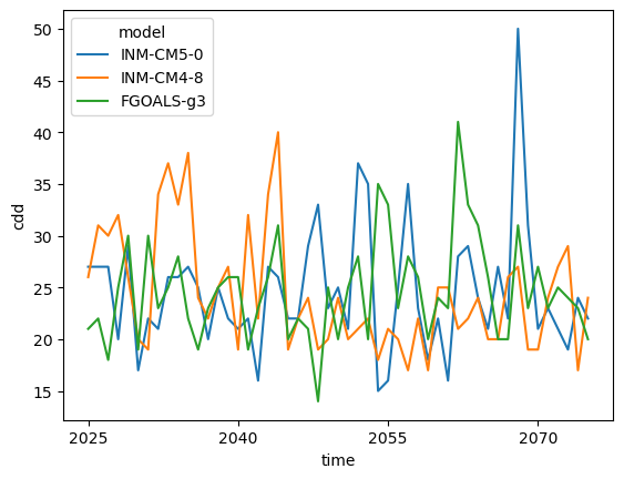
There is a lot of variation in the 3 models over time, so let’s plot the general mean
trend, with error bands. We will convert the data from an xarray.Dataset to a
pandas.DataFrame table before making this plot.
# Convert CFTime to Python datetime
if cdd_mean.time.dtype == "object":
    cdd_mean["time"] = cdd_mean.indexes["time"].to_datetimeindex(time_unit="s")

# Convert from xarray.Dataset to pandas.DataFrame
df_cdd = cdd_mean.to_pandas().T

# Save to csv file (optional)
df_cdd.to_csv(path_or_buf=f"vut_consecutive_dry_days_{SSP_ID}.csv")

df_cdd.head()
/tmp/ipykernel_2725/1597848363.py:3: RuntimeWarning: Converting a CFTimeIndex with dates from a non-standard calendar, 'noleap', to a pandas.DatetimeIndex, which uses dates from the standard calendar. This may lead to subtle errors in operations that depend on the length of time between dates.
cdd_mean["time"] = cdd_mean.indexes["time"].to_datetimeindex(time_unit="s")
# Collapse or melt many columns (models) into one column
df_cdd2 = df_cdd.melt(ignore_index=False)
df_cdd2sns.relplot(data=df_cdd2, x="time", y="value", kind="line")<seaborn.axisgrid.FacetGrid at 0x7f0dedf97790>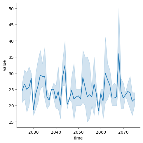
That’s all! Hopefully this will get you started on how to handle CMIP6 climate data!
- Gergel, D. R., Malevich, S. B., McCusker, K. E., Tenezakis, E., Delgado, M. T., Fish, M. A., & Kopp, R. E. (2024). Global Downscaled Projections for Climate Impacts Research (GDPCIR): preserving quantile trends for modeling future climate impacts. Geoscientific Model Development, 17(1), 191–227. 10.5194/gmd-17-191-2024