Predicting flood risk with ERA5 Climate Reanalysis and Elevation data in Vanuatu
In this lesson, we will use historic ERA5 Land data and a Digital Elevation Model to predict a flood event. The core components will entail learning about ERA5 data, how to construct flood proxy labels based on physically and empirically established thresholds for likely flood events, and train a model to learn from these proxy labels over a time series to infer flood events in new data.
import glob
import numpy as np
import xarray as xr
import hvplot.xarray
import hvplot.pandas
import holoviews as hv
import planetary_computer
from holoviews import opts
from holoviews.element import tiles
import cartopy.crs as ccrs
import cartopy.crs as ccrs
import cartopy.feature as cfeature
import matplotlib.pyplot as plt
from pystac_client import Client
import odc.stac
from shapely.geometry import Polygon, MultiPolygon, box
from shapely.ops import unary_union
import rioxarray as rxr
import pandas as pd
import geopandas as gpd
from sklearn.metrics import classification_report
from sklearn.ensemble import RandomForestClassifier
from sklearn.metrics import accuracy_score, ConfusionMatrixDisplay
from sklearn.model_selection import train_test_split
#from cuml import RandomForestClassifier
#import cupy as cp
#from cupyx.scipy.ndimage import convolve
#from dask import compute, delayed
#from dask_ml.model_selection import train_test_split
from rasterio.enums import Resamplingxr.set_options(keep_attrs=True)<xarray.core.options.set_options at 0x7f57ec098eb0>Let’s read in the administrative boundaries. We’ll use these for visualizing land boundaries and subsetting data.
admin_boundaries_gdf = gpd.read_file("./2016_phc_vut_pid_4326.geojson")
admin_boundaries_gdf = admin_boundaries_gdf.set_index(keys="pname")  # set province name as the index
Next we’ll obtain ground truth flood masks, the same as used in Lesson 1C from the Tropical and Sub-Tropical Flood and Water Masks dataset. We’ll use these to determine how well we can predict a historic flood event.
# Download the data (subset_vbos_smaller.zip)
!gdown "https://drive.google.com/uc?id=1rLNwGQf8C93CXpdQ293zKaKiQejDdJnp"
# Unzip the compressed data
!mkdir -p flood/
!unzip subset_vbos_smaller.zip -d flood/ls flood/subset_vbos_smaller/2016_phc_vut_iid_4326.geojson metadata/
final_model_20ep.pth tst-ground-truth-flood-masks/
# Get list of all labels
mask_paths = glob.glob('flood/subset_vbos_smaller/tst-ground-truth-flood-masks/*.tif')len(mask_paths)34Filter for flood events only in Vanuatu.
df = pd.read_csv('flood/subset_vbos_smaller/metadata/metadata.csv')
# Filter for specific countries
# Ensure the column is in datetime format
df["event_date"] = pd.to_datetime(df["Event Date"], format="%m/%d/%Y", errors="coerce")

# Filter for rows where the year is 2020
#df_2020 = df[df["event_date"].dt.year == 2020]
#print(len(df_2020))

selected_countries = {"Vanuatu"} #, "Timor-Leste" , "Philippines"} #, "Viet Nam", "Australia"}
df = df[df["Country"].isin(selected_countries)]

print("len(df):", len(df))
len(df): 1
dfAs a reminder, the metadata entails:
Activation Date: Date when the flood event was registered in the EMS Rapid Mapping system.
Event Date: Initial date of the flood occurrence.
Satellite Date: Date of the latest satellite imagery used for generating the flood mask.
The classes and therefore pixel values available in the images entail:
0: No data
1: Land (not flooded)
2: Flooded areas
3: Permanent water bodies
ls flood/subset_vbos_smaller/tst-ground-truth-flood-masks/EMSR434_AOI05_GRA_PRODUCT_ground_truth.tifflood/subset_vbos_smaller/tst-ground-truth-flood-masks/EMSR434_AOI05_GRA_PRODUCT_ground_truth.tif
Read in the available flood ground truth mask image.
# Read the flood mask as a DataArray
flood_mask = rxr.open_rasterio(
    "flood/subset_vbos_smaller/tst-ground-truth-flood-masks/EMSR434_AOI05_GRA_PRODUCT_ground_truth.tif",
    masked=True # masks no data values
).squeeze("band") # Remove band dimension if only 1 bandnp.unique(flood_mask.data)array([0., 1., 2., 3.], dtype=float32)flood_mask.plot.imshow(cmap="Blues")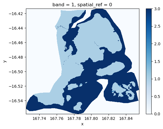
Plot the province that overlaps with the ground truth flood mask.
flood_mask.rio.crsCRS.from_wkt('GEOGCS["WGS 84",DATUM["WGS_1984",SPHEROID["WGS 84",6378137,298.257223563,AUTHORITY["EPSG","7030"]],AUTHORITY["EPSG","6326"]],PRIMEM["Greenwich",0,AUTHORITY["EPSG","8901"]],UNIT["degree",0.0174532925199433,AUTHORITY["EPSG","9122"]],AXIS["Latitude",NORTH],AXIS["Longitude",EAST],AUTHORITY["EPSG","4326"]]')# Reproject vector data to match flood_mask CRS
if hasattr(flood_mask, 'rio') and flood_mask.rio.crs is not None:
admin_boundaries_gdf = admin_boundaries_gdf.to_crs(flood_mask.rio.crs)
fig, ax = plt.subplots(figsize=(10, 8))
# MALAMPA boundary (the province which overlaps witht he flood mask)
malampa_geom = admin_boundaries_gdf.loc["MALAMPA"]
malampa_gdf = gpd.GeoDataFrame(geometry=[malampa_geom.geometry], crs=admin_boundaries_gdf.crs)
malampa_gdf.boundary.plot(ax=ax, edgecolor='green', linewidth=2, label="Boundary of Malampa")
# Plot the bounding box of Malampa
minx, miny, maxx, maxy = malampa_gdf.total_bounds
bbox_geom = box(minx, miny, maxx, maxy)
bbox_gdf = gpd.GeoDataFrame(geometry=[bbox_geom], crs=malampa_gdf.crs)
minx, miny, maxx, maxy = bbox_gdf.total_bounds
ax.set_xlim(minx - 0.1, maxx + 0.1)
ax.set_ylim(miny - 0.1, maxy + 0.1)
bbox_gdf.boundary.plot(ax=ax, edgecolor='red', linewidth=2, label="Bounding Box of Malampa")
# Plot flood mask on top
flood_mask.plot.imshow(ax=ax, cmap="Blues", alpha=0.6, add_colorbar=True)
plt.title("Flood Mask on Top of Bounding Box and MALAMPA Boundary")
plt.legend()
plt.tight_layout()
plt.show()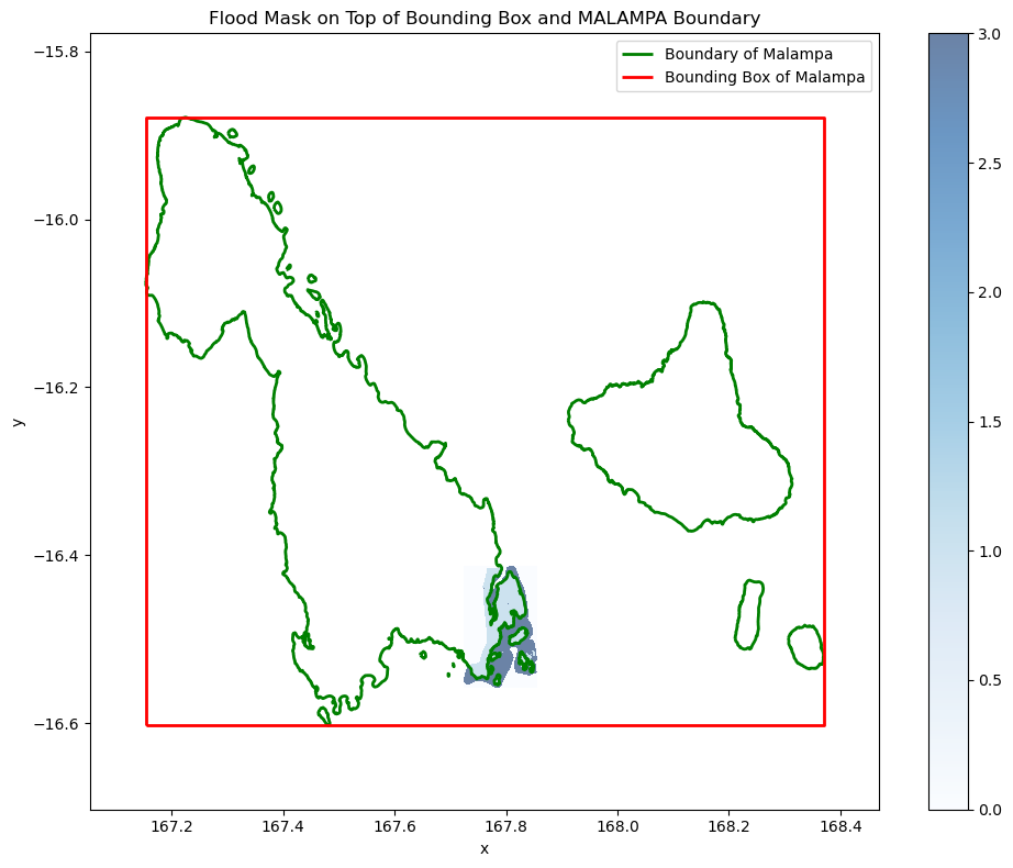
Get the bounds of the province.
minx, miny, maxx, maxy = malampa_gdf.total_bounds

# Latitude decreases as you go south, so maxy is the northern bound and miny the southern
lat_slice = slice(maxy, miny)   # from north to south
lon_slice = slice(minx, maxx)   # from west to east

# Bounding box for Malampa largest island
print("lat_slice:", lat_slice)
print("lon_slice:", lon_slice)
lat_slice: slice(-15.878752595167615, -16.602589224766035, None)
lon_slice: slice(167.15336525903868, 168.36996267483048, None)
Now, we need to sign up for an account on Destination Earth platform. Once you’ve done that, go to Earth Data Hub account settings, copy your default personal access token or create a new one and paste it below.
PAT = "edh_pat_..."Let’s open the ERA5-Land hourly data.
ERA5-Land is a global hourly reanalysis dataset produced by the European Centre for Medium-Range Weather Forecasts (ECMWF) as part of the Copernicus Climate Change Service (C3S).
It provides ∼9 km land-surface weather and climate variables from January 1950 to near-real-time, and is tailored for applications that need detailed land surface information — like flood modeling.
Reanalysis data combines historical observations (satellite, in-situ, weather stations) with a numerical weather prediction model to produce consistent, gap-free datasets of atmospheric and land-surface variables. This provides physically consistent gridded data across time and space, making it ideal for long-term analysis and climate studies. Think of it as creating a best-estimate “weather reconstruction” using all available observations and physics-based modeling.
Some useful variables for flood prediction:
| Category | Variables | Units |
|---|---|---|
| Precipitation | tp | m/hour |
| Soil moisture | swvl1-4 | m³/m³ (volume/volume) |
| Runoff | ro | m/hour |
| Potential evaporation | pev | m/hour |
Why Is ERA5-Land Useful for Flood Prediction?
Rainfall Forcing:
Hourly total_precipitation gives rainfall estimates — a key input for hydrological models.
Soil Moisture Saturation:
Soil moisture layers help determine how saturated the ground is — saturated soils lead to increased runoff and flash flooding.
Surface & Subsurface Runoff:
These variables indicate how water is moving through and over the landscape, critical for identifying flood-prone zones.
Long-Term Trends:
Being available since 1950, ERA5-Land is valuable for:
Understanding historic flood events
Training machine learning flood prediction models
Detecting changes in hydrological regimes
ds = xr.open_dataset(
    f"https://edh:{PAT}@data.earthdatahub.destine.eu/era5/reanalysis-era5-land-no-antartica-v0.zarr",
    chunks={},
    engine="zarr",
)
ds
/srv/conda/envs/notebook/lib/python3.10/site-packages/xarray_sentinel/esa_safe.py:7: UserWarning: pkg_resources is deprecated as an API. See https://setuptools.pypa.io/en/latest/pkg_resources.html. The pkg_resources package is slated for removal as early as 2025-11-30. Refrain from using this package or pin to Setuptools<81.
import pkg_resources
ds.data_varsData variables:
asn (valid_time, latitude, longitude) float32 14TB dask.array<chunksize=(2880, 64, 64), meta=np.ndarray>
d2m (valid_time, latitude, longitude) float32 14TB dask.array<chunksize=(2880, 64, 64), meta=np.ndarray>
e (valid_time, latitude, longitude) float32 14TB dask.array<chunksize=(2880, 64, 64), meta=np.ndarray>
es (valid_time, latitude, longitude) float32 14TB dask.array<chunksize=(2880, 64, 64), meta=np.ndarray>
evabs (valid_time, latitude, longitude) float32 14TB dask.array<chunksize=(2880, 64, 64), meta=np.ndarray>
evaow (valid_time, latitude, longitude) float32 14TB dask.array<chunksize=(2880, 64, 64), meta=np.ndarray>
evatc (valid_time, latitude, longitude) float32 14TB dask.array<chunksize=(2880, 64, 64), meta=np.ndarray>
evavt (valid_time, latitude, longitude) float32 14TB dask.array<chunksize=(2880, 64, 64), meta=np.ndarray>
fal (valid_time, latitude, longitude) float32 14TB dask.array<chunksize=(2880, 64, 64), meta=np.ndarray>
lai_hv (valid_time, latitude, longitude) float32 14TB dask.array<chunksize=(2880, 64, 64), meta=np.ndarray>
lai_lv (valid_time, latitude, longitude) float32 14TB dask.array<chunksize=(2880, 64, 64), meta=np.ndarray>
lblt (valid_time, latitude, longitude) float32 14TB dask.array<chunksize=(2880, 64, 64), meta=np.ndarray>
licd (valid_time, latitude, longitude) float32 14TB dask.array<chunksize=(2880, 64, 64), meta=np.ndarray>
lict (valid_time, latitude, longitude) float32 14TB dask.array<chunksize=(2880, 64, 64), meta=np.ndarray>
lmld (valid_time, latitude, longitude) float32 14TB dask.array<chunksize=(2880, 64, 64), meta=np.ndarray>
lmlt (valid_time, latitude, longitude) float32 14TB dask.array<chunksize=(2880, 64, 64), meta=np.ndarray>
lshf (valid_time, latitude, longitude) float32 14TB dask.array<chunksize=(2880, 64, 64), meta=np.ndarray>
ltlt (valid_time, latitude, longitude) float32 14TB dask.array<chunksize=(2880, 64, 64), meta=np.ndarray>
pev (valid_time, latitude, longitude) float32 14TB dask.array<chunksize=(2880, 64, 64), meta=np.ndarray>
ro (valid_time, latitude, longitude) float32 14TB dask.array<chunksize=(2880, 64, 64), meta=np.ndarray>
rsn (valid_time, latitude, longitude) float32 14TB dask.array<chunksize=(2880, 64, 64), meta=np.ndarray>
sd (valid_time, latitude, longitude) float32 14TB dask.array<chunksize=(2880, 64, 64), meta=np.ndarray>
sde (valid_time, latitude, longitude) float32 14TB dask.array<chunksize=(2880, 64, 64), meta=np.ndarray>
sf (valid_time, latitude, longitude) float32 14TB dask.array<chunksize=(2880, 64, 64), meta=np.ndarray>
skt (valid_time, latitude, longitude) float32 14TB dask.array<chunksize=(2880, 64, 64), meta=np.ndarray>
slhf (valid_time, latitude, longitude) float32 14TB dask.array<chunksize=(2880, 64, 64), meta=np.ndarray>
smlt (valid_time, latitude, longitude) float32 14TB dask.array<chunksize=(2880, 64, 64), meta=np.ndarray>
snowc (valid_time, latitude, longitude) float32 14TB dask.array<chunksize=(2880, 64, 64), meta=np.ndarray>
sp (valid_time, latitude, longitude) float32 14TB dask.array<chunksize=(2880, 64, 64), meta=np.ndarray>
src (valid_time, latitude, longitude) float32 14TB dask.array<chunksize=(2880, 64, 64), meta=np.ndarray>
sro (valid_time, latitude, longitude) float32 14TB dask.array<chunksize=(2880, 64, 64), meta=np.ndarray>
sshf (valid_time, latitude, longitude) float32 14TB dask.array<chunksize=(2880, 64, 64), meta=np.ndarray>
ssr (valid_time, latitude, longitude) float32 14TB dask.array<chunksize=(2880, 64, 64), meta=np.ndarray>
ssrd (valid_time, latitude, longitude) float32 14TB dask.array<chunksize=(2880, 64, 64), meta=np.ndarray>
ssro (valid_time, latitude, longitude) float32 14TB dask.array<chunksize=(2880, 64, 64), meta=np.ndarray>
stl1 (valid_time, latitude, longitude) float32 14TB dask.array<chunksize=(2880, 64, 64), meta=np.ndarray>
stl2 (valid_time, latitude, longitude) float32 14TB dask.array<chunksize=(2880, 64, 64), meta=np.ndarray>
stl3 (valid_time, latitude, longitude) float32 14TB dask.array<chunksize=(2880, 64, 64), meta=np.ndarray>
stl4 (valid_time, latitude, longitude) float32 14TB dask.array<chunksize=(2880, 64, 64), meta=np.ndarray>
str (valid_time, latitude, longitude) float32 14TB dask.array<chunksize=(2880, 64, 64), meta=np.ndarray>
strd (valid_time, latitude, longitude) float32 14TB dask.array<chunksize=(2880, 64, 64), meta=np.ndarray>
swvl1 (valid_time, latitude, longitude) float32 14TB dask.array<chunksize=(2880, 64, 64), meta=np.ndarray>
swvl2 (valid_time, latitude, longitude) float32 14TB dask.array<chunksize=(2880, 64, 64), meta=np.ndarray>
swvl3 (valid_time, latitude, longitude) float32 14TB dask.array<chunksize=(2880, 64, 64), meta=np.ndarray>
swvl4 (valid_time, latitude, longitude) float32 14TB dask.array<chunksize=(2880, 64, 64), meta=np.ndarray>
t2m (valid_time, latitude, longitude) float32 14TB dask.array<chunksize=(2880, 64, 64), meta=np.ndarray>
tp (valid_time, latitude, longitude) float32 14TB dask.array<chunksize=(2880, 64, 64), meta=np.ndarray>
tsn (valid_time, latitude, longitude) float32 14TB dask.array<chunksize=(2880, 64, 64), meta=np.ndarray>
u10 (valid_time, latitude, longitude) float32 14TB dask.array<chunksize=(2880, 64, 64), meta=np.ndarray>
v10 (valid_time, latitude, longitude) float32 14TB dask.array<chunksize=(2880, 64, 64), meta=np.ndarray>Let’s select our key variables for flood prediction. Multiplying the units by 1000 is done to convert units from meters (m) or cubic meters per cubic meter (m³/m³) into millimeters (mm) — a much more intuitive and commonly used unit in hydrology and flood studies.
# Load ERA5 dataset
# Variables: ds.tp, ds.swvl1, ds.swvl2, ds.ro, ds.msl

# Convert units and subset
tp_mm = ds.tp * 1000  # m → mm
tp_mm.attrs["units"] = "mm"
tp_mm_vanu = tp_mm.sel(latitude=lat_slice, longitude=lon_slice)

swvl1_mm = ds.swvl1 * 1000  # m³/m³ → mm
swvl1_mm.attrs["units"] = "mm"
swvl1_vanu = swvl1_mm.sel(latitude=lat_slice, longitude=lon_slice)

swvl2_mm = ds.swvl2 * 1000
swvl2_mm.attrs["units"] = "mm"
swvl2_vanu = swvl2_mm.sel(latitude=lat_slice, longitude=lon_slice)

ro_mm = ds.ro * 1000  # m → mm
ro_mm.attrs["units"] = "mm"
ro_vanu = ro_mm.sel(latitude=lat_slice, longitude=lon_slice)

pev_mm = ds.pev * 1000  # m/day → mm/day
pev_mm.attrs["units"] = "mm/day"
pev_vanu = pev_mm.sel(latitude=lat_slice, longitude=lon_slice)

# Combine into a composite xarray Dataset
flood_composite = xr.Dataset({
    "precip_mm": tp_mm_vanu,
    "soil_moisture_l1_mm": swvl1_vanu,
    "soil_moisture_l2_mm": swvl2_vanu,
    "runoff_mm": ro_vanu,
    "potential_evaporation_mm_day": pev_vanu,
})

flood_compositeLet’s get a snapshot of the variables on the date of a historic flood event: Tropical cyclone Harold on April 7, 2020. This is the approximately date of the flood mask we selected earlier.
flood_composite_04072020 = flood_composite.sel(
    valid_time="2020-04-07"
)

flood_composite_04072020Notice thar there are 24 time steps available for April 7, 2020. This makes sense as this is hourly data over the course of one day.
flood_composite_04072020Let’s also obtain data for all of 2020 and 2021. We’ll use this to train a model to learn patterns associated with potential flood events from a time series.
# Select only the year 2020
flood_composite_2020 = flood_composite.sel(
    valid_time=slice('2020', '2020')
)

flood_composite_2020# Select only the year 2021
flood_composite_2021 = flood_composite.sel(
valid_time=slice('2021', '2021')
)
flood_composite_2021Let’s plot total precipitation for April 7, 2020.
hv.extension('bokeh')

proj = ccrs.Mercator.GOOGLE
precip_plot = flood_composite_04072020["precip_mm"].hvplot(
    x='longitude',
    y='latitude',
    geo=True,
    cmap='Blues_r',
    clim=(0, 400),
    title="Total precipitation 04/07/2020",
    frame_width=600,
    colorbar=True,
)

# Add basemap and set projection globally
basemap = tiles.OSM().opts(alpha=0.5)

combined = (precip_plot * basemap).opts(
    opts.Overlay(
        projection=proj,
        global_extent=False,
        frame_width=600
    )
)

combinedAborting load due to failure while reading: https://nasademeuwest.blob.core.windows.net/nasadem-cog/v001/NASADEM_HGT_s17e168.tif?st=2025-08-09T10%3A05%3A53Z&se=2025-08-10T10%3A50%3A53Z&sp=rl&sv=2025-07-05&sr=c&skoid=9c8ff44a-6a2c-4dfb-b298-1c9212f64d9a&sktid=72f988bf-86f1-41af-91ab-2d7cd011db47&skt=2025-08-10T00%3A02%3A21Z&ske=2025-08-17T00%3A02%3A21Z&sks=b&skv=2025-07-05&sig=O3jKAYlLSMaVte3qCE20EtFgjcqhigG5fhfYKPVlMmo%3D:1
Aborting load due to failure while reading: https://nasademeuwest.blob.core.windows.net/nasadem-cog/v001/NASADEM_HGT_s17e168.tif?st=2025-08-09T10%3A05%3A53Z&se=2025-08-10T10%3A50%3A53Z&sp=rl&sv=2025-07-05&sr=c&skoid=9c8ff44a-6a2c-4dfb-b298-1c9212f64d9a&sktid=72f988bf-86f1-41af-91ab-2d7cd011db47&skt=2025-08-10T00%3A02%3A21Z&ske=2025-08-17T00%3A02%3A21Z&sks=b&skv=2025-07-05&sig=O3jKAYlLSMaVte3qCE20EtFgjcqhigG5fhfYKPVlMmo%3D:1
Aborting load due to failure while reading: https://nasademeuwest.blob.core.windows.net/nasadem-cog/v001/NASADEM_HGT_s17e168.tif?st=2025-08-09T10%3A05%3A53Z&se=2025-08-10T10%3A50%3A53Z&sp=rl&sv=2025-07-05&sr=c&skoid=9c8ff44a-6a2c-4dfb-b298-1c9212f64d9a&sktid=72f988bf-86f1-41af-91ab-2d7cd011db47&skt=2025-08-10T00%3A02%3A21Z&ske=2025-08-17T00%3A02%3A21Z&sks=b&skv=2025-07-05&sig=O3jKAYlLSMaVte3qCE20EtFgjcqhigG5fhfYKPVlMmo%3D:1
Aborting load due to failure while reading: https://nasademeuwest.blob.core.windows.net/nasadem-cog/v001/NASADEM_HGT_s17e168.tif?st=2025-08-09T10%3A05%3A53Z&se=2025-08-10T10%3A50%3A53Z&sp=rl&sv=2025-07-05&sr=c&skoid=9c8ff44a-6a2c-4dfb-b298-1c9212f64d9a&sktid=72f988bf-86f1-41af-91ab-2d7cd011db47&skt=2025-08-10T00%3A02%3A21Z&ske=2025-08-17T00%3A02%3A21Z&sks=b&skv=2025-07-05&sig=O3jKAYlLSMaVte3qCE20EtFgjcqhigG5fhfYKPVlMmo%3D:1
/srv/conda/envs/notebook/lib/python3.10/site-packages/dask/array/numpy_compat.py:57: RuntimeWarning: invalid value encountered in divide
x = np.divide(x1, x2, out)
/srv/conda/envs/notebook/lib/python3.10/site-packages/dask/array/numpy_compat.py:57: RuntimeWarning: invalid value encountered in divide
x = np.divide(x1, x2, out)
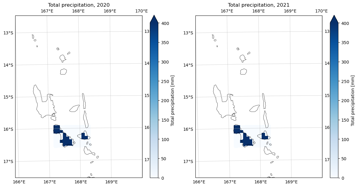
Let’s also plot annually summed total precipitation for 2020 and 2021.
def plot_xarray_maps(datasets, titles=None, projection=ccrs.UTM(zone=59, southern_hemisphere=True), vmax=None, cmap='Blues'):
"""
Plot multiple xarray 2D datasets.
Zooms into Vanuatu region.
"""
n = len(datasets)
fig, axs = plt.subplots(1, n, figsize=(6 * n, 6),
subplot_kw={'projection': projection})
if n == 1:
axs = [axs]
for i, (data, ax) in enumerate(zip(datasets, axs)):
im = data.plot.imshow(
ax=ax,
transform=ccrs.PlateCarree(),
cmap=cmap,
vmax=vmax,
add_colorbar=True
)
# Try to set extent from data bounds if available
try:
lon_min = float(data.lon.min())
lon_max = float(data.lon.max())
lat_min = float(data.lat.min())
lat_max = float(data.lat.max())
ax.set_extent([lon_min, lon_max, lat_min, lat_max], crs=ccrs.PlateCarree())
except Exception:
# Fallback to manual Vanuatu bounding box
ax.set_extent([166, 170, -17.5, -12.5], crs=ccrs.PlateCarree())
ax.coastlines(resolution='10m', linewidth=0.5)
ax.add_feature(cfeature.BORDERS, linewidth=0.3)
ax.set_title(titles[i] if titles else f"Map {i+1}")
ax.gridlines(draw_labels=True, alpha=0.5)
plt.tight_layout()
plt.show()
plot_xarray_maps(
datasets=[flood_composite_2020["precip_mm"].sum("valid_time"), flood_composite_2021["precip_mm"].sum("valid_time")],
titles=[
"Total precipitation, 2020",
"Total precipitation, 2021"
],
projection=ccrs.UTM(zone=59, southern_hemisphere=True),
vmax=400,
cmap="Blues"
)
Aborting load due to failure while reading: https://nasademeuwest.blob.core.windows.net/nasadem-cog/v001/NASADEM_HGT_s17e168.tif?st=2025-08-09T10%3A05%3A53Z&se=2025-08-10T10%3A50%3A53Z&sp=rl&sv=2025-07-05&sr=c&skoid=9c8ff44a-6a2c-4dfb-b298-1c9212f64d9a&sktid=72f988bf-86f1-41af-91ab-2d7cd011db47&skt=2025-08-10T00%3A02%3A21Z&ske=2025-08-17T00%3A02%3A21Z&sks=b&skv=2025-07-05&sig=O3jKAYlLSMaVte3qCE20EtFgjcqhigG5fhfYKPVlMmo%3D:1
Aborting load due to failure while reading: https://nasademeuwest.blob.core.windows.net/nasadem-cog/v001/NASADEM_HGT_s17e168.tif?st=2025-08-09T10%3A05%3A53Z&se=2025-08-10T10%3A50%3A53Z&sp=rl&sv=2025-07-05&sr=c&skoid=9c8ff44a-6a2c-4dfb-b298-1c9212f64d9a&sktid=72f988bf-86f1-41af-91ab-2d7cd011db47&skt=2025-08-10T00%3A02%3A21Z&ske=2025-08-17T00%3A02%3A21Z&sks=b&skv=2025-07-05&sig=O3jKAYlLSMaVte3qCE20EtFgjcqhigG5fhfYKPVlMmo%3D:1
Aborting load due to failure while reading: https://nasademeuwest.blob.core.windows.net/nasadem-cog/v001/NASADEM_HGT_s17e168.tif?st=2025-08-09T10%3A05%3A53Z&se=2025-08-10T10%3A50%3A53Z&sp=rl&sv=2025-07-05&sr=c&skoid=9c8ff44a-6a2c-4dfb-b298-1c9212f64d9a&sktid=72f988bf-86f1-41af-91ab-2d7cd011db47&skt=2025-08-10T00%3A02%3A21Z&ske=2025-08-17T00%3A02%3A21Z&sks=b&skv=2025-07-05&sig=O3jKAYlLSMaVte3qCE20EtFgjcqhigG5fhfYKPVlMmo%3D:1
Aborting load due to failure while reading: https://nasademeuwest.blob.core.windows.net/nasadem-cog/v001/NASADEM_HGT_s17e168.tif?st=2025-08-09T10%3A05%3A53Z&se=2025-08-10T10%3A50%3A53Z&sp=rl&sv=2025-07-05&sr=c&skoid=9c8ff44a-6a2c-4dfb-b298-1c9212f64d9a&sktid=72f988bf-86f1-41af-91ab-2d7cd011db47&skt=2025-08-10T00%3A02%3A21Z&ske=2025-08-17T00%3A02%3A21Z&sks=b&skv=2025-07-05&sig=O3jKAYlLSMaVte3qCE20EtFgjcqhigG5fhfYKPVlMmo%3D:1
Aborting load due to failure while reading: https://nasademeuwest.blob.core.windows.net/nasadem-cog/v001/NASADEM_HGT_s17e168.tif?st=2025-08-09T10%3A05%3A53Z&se=2025-08-10T10%3A50%3A53Z&sp=rl&sv=2025-07-05&sr=c&skoid=9c8ff44a-6a2c-4dfb-b298-1c9212f64d9a&sktid=72f988bf-86f1-41af-91ab-2d7cd011db47&skt=2025-08-10T00%3A02%3A21Z&ske=2025-08-17T00%3A02%3A21Z&sks=b&skv=2025-07-05&sig=O3jKAYlLSMaVte3qCE20EtFgjcqhigG5fhfYKPVlMmo%3D:1
Aborting load due to failure while reading: https://nasademeuwest.blob.core.windows.net/nasadem-cog/v001/NASADEM_HGT_s17e168.tif?st=2025-08-09T10%3A05%3A53Z&se=2025-08-10T10%3A50%3A53Z&sp=rl&sv=2025-07-05&sr=c&skoid=9c8ff44a-6a2c-4dfb-b298-1c9212f64d9a&sktid=72f988bf-86f1-41af-91ab-2d7cd011db47&skt=2025-08-10T00%3A02%3A21Z&ske=2025-08-17T00%3A02%3A21Z&sks=b&skv=2025-07-05&sig=O3jKAYlLSMaVte3qCE20EtFgjcqhigG5fhfYKPVlMmo%3D:1
Aborting load due to failure while reading: https://nasademeuwest.blob.core.windows.net/nasadem-cog/v001/NASADEM_HGT_s17e168.tif?st=2025-08-09T10%3A05%3A53Z&se=2025-08-10T10%3A50%3A53Z&sp=rl&sv=2025-07-05&sr=c&skoid=9c8ff44a-6a2c-4dfb-b298-1c9212f64d9a&sktid=72f988bf-86f1-41af-91ab-2d7cd011db47&skt=2025-08-10T00%3A02%3A21Z&ske=2025-08-17T00%3A02%3A21Z&sks=b&skv=2025-07-05&sig=O3jKAYlLSMaVte3qCE20EtFgjcqhigG5fhfYKPVlMmo%3D:1
Aborting load due to failure while reading: https://nasademeuwest.blob.core.windows.net/nasadem-cog/v001/NASADEM_HGT_s17e168.tif?st=2025-08-09T10%3A05%3A53Z&se=2025-08-10T10%3A50%3A53Z&sp=rl&sv=2025-07-05&sr=c&skoid=9c8ff44a-6a2c-4dfb-b298-1c9212f64d9a&sktid=72f988bf-86f1-41af-91ab-2d7cd011db47&skt=2025-08-10T00%3A02%3A21Z&ske=2025-08-17T00%3A02%3A21Z&sks=b&skv=2025-07-05&sig=O3jKAYlLSMaVte3qCE20EtFgjcqhigG5fhfYKPVlMmo%3D:1
Aborting load due to failure while reading: https://nasademeuwest.blob.core.windows.net/nasadem-cog/v001/NASADEM_HGT_s17e168.tif?st=2025-08-09T10%3A05%3A53Z&se=2025-08-10T10%3A50%3A53Z&sp=rl&sv=2025-07-05&sr=c&skoid=9c8ff44a-6a2c-4dfb-b298-1c9212f64d9a&sktid=72f988bf-86f1-41af-91ab-2d7cd011db47&skt=2025-08-10T00%3A02%3A21Z&ske=2025-08-17T00%3A02%3A21Z&sks=b&skv=2025-07-05&sig=O3jKAYlLSMaVte3qCE20EtFgjcqhigG5fhfYKPVlMmo%3D:1
Aborting load due to failure while reading: https://nasademeuwest.blob.core.windows.net/nasadem-cog/v001/NASADEM_HGT_s17e168.tif?st=2025-08-09T10%3A05%3A53Z&se=2025-08-10T10%3A50%3A53Z&sp=rl&sv=2025-07-05&sr=c&skoid=9c8ff44a-6a2c-4dfb-b298-1c9212f64d9a&sktid=72f988bf-86f1-41af-91ab-2d7cd011db47&skt=2025-08-10T00%3A02%3A21Z&ske=2025-08-17T00%3A02%3A21Z&sks=b&skv=2025-07-05&sig=O3jKAYlLSMaVte3qCE20EtFgjcqhigG5fhfYKPVlMmo%3D:1
Aborting load due to failure while reading: https://nasademeuwest.blob.core.windows.net/nasadem-cog/v001/NASADEM_HGT_s17e168.tif?st=2025-08-09T10%3A05%3A53Z&se=2025-08-10T10%3A50%3A53Z&sp=rl&sv=2025-07-05&sr=c&skoid=9c8ff44a-6a2c-4dfb-b298-1c9212f64d9a&sktid=72f988bf-86f1-41af-91ab-2d7cd011db47&skt=2025-08-10T00%3A02%3A21Z&ske=2025-08-17T00%3A02%3A21Z&sks=b&skv=2025-07-05&sig=O3jKAYlLSMaVte3qCE20EtFgjcqhigG5fhfYKPVlMmo%3D:1
Aborting load due to failure while reading: https://nasademeuwest.blob.core.windows.net/nasadem-cog/v001/NASADEM_HGT_s17e168.tif?st=2025-08-09T10%3A05%3A53Z&se=2025-08-10T10%3A50%3A53Z&sp=rl&sv=2025-07-05&sr=c&skoid=9c8ff44a-6a2c-4dfb-b298-1c9212f64d9a&sktid=72f988bf-86f1-41af-91ab-2d7cd011db47&skt=2025-08-10T00%3A02%3A21Z&ske=2025-08-17T00%3A02%3A21Z&sks=b&skv=2025-07-05&sig=O3jKAYlLSMaVte3qCE20EtFgjcqhigG5fhfYKPVlMmo%3D:1
/srv/conda/envs/notebook/lib/python3.10/site-packages/dask/array/numpy_compat.py:57: RuntimeWarning: invalid value encountered in divide
  x = np.divide(x1, x2, out)
/srv/conda/envs/notebook/lib/python3.10/site-packages/dask/array/numpy_compat.py:57: RuntimeWarning: invalid value encountered in divide
  x = np.divide(x1, x2, out)
Differences between the two years aren’t well highlighted in those plots, so we can print the maximum pixel value from the annual numerical sums as well as plot the total precipitation time series for each year as well.
flood_composite_2020["precip_mm"].sum("valid_time").values.max(), flood_composite_2021["precip_mm"].sum("valid_time").values.max()(36744.305, 36370.43)# Spatial average over lat and lon dims
flood_composite_2020_mean = flood_composite_2020["precip_mm"].mean(dim=['latitude', 'longitude'])
flood_composite_2021_mean = flood_composite_2021["precip_mm"].mean(dim=['latitude', 'longitude'])
plt.style.use('fivethirtyeight')
fig, ax = plt.subplots(figsize=(10,6))
ax.plot(flood_composite_2020_mean['valid_time'], flood_composite_2020_mean.values, label='2020 Accumulated Precipitation', linewidth=2)
ax.plot(flood_composite_2021_mean['valid_time'], flood_composite_2021_mean.values, label='2021 Accumulated Precipitation', linewidth=2)
ax.set_ylim([-100, 1750])
ax.set_title('Accumulated precipitation [mm], Vanuatu (Approximate bbox)', loc='left', fontsize=14)
ax.set_xlabel('Time')
ax.set_ylabel('Precipitation (mm)')
ax.legend(prop={'size': 10})
plt.show()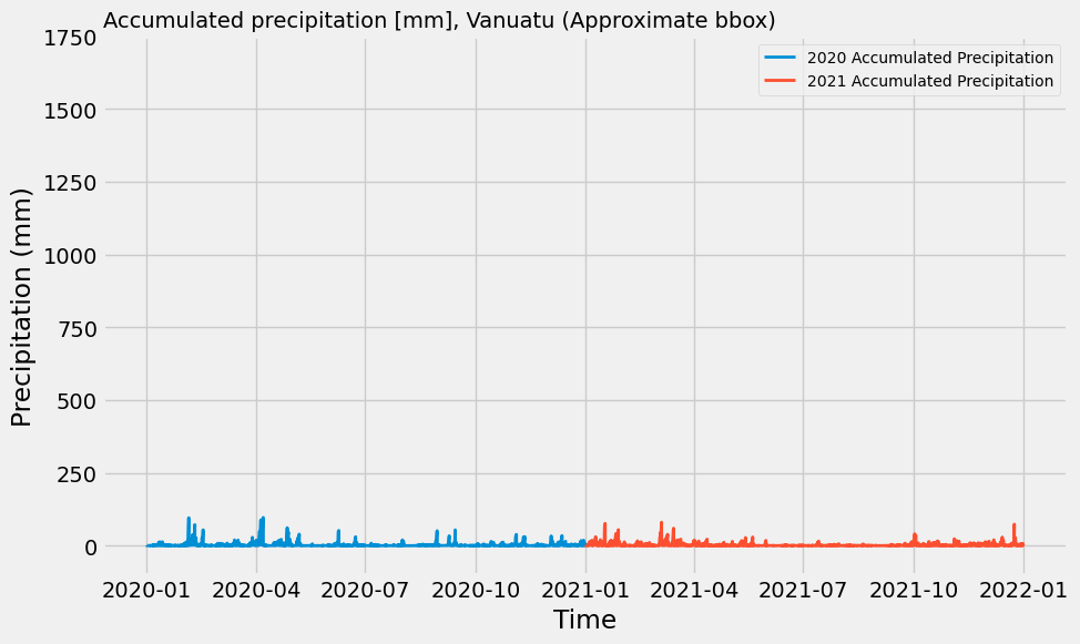
flood_composite_04072020 = flood_composite_04072020.rio.write_crs("EPSG:4326")
flood_composite_2020 = flood_composite_2020.rio.write_crs("EPSG:4326")
flood_composite_2021 = flood_composite_2021.rio.write_crs("EPSG:4326")
Now we will acquire a Digital Elevation Model. The one we will use is the NASA DEM, which features ~30 meter horizontal resolution, and is primarily derived from the Shuttle Radar Topography Mission (SRTM). The SRTM mission used C-band SAR as its primary instrument (with some X-band coverage from a second instrument). C-band penetrates vegetation canopy more than X-band, but less than L-band. In forested or shrub-covered areas, the radar signal often reflects from the top of canopy or upper branches, not the bare ground. This means the NASADEM elevations are Digital Surface Model (DSM) heights, not actual ground. For flood modeling, it may slightly overestimate ground elevation by underestimating flood depth or flood extent in vegetated zones. In urban areas, C-band reflects strongly off rooftops, walls, and elevated surfaces. This again raises the measured “ground” elevation above the real surface and could make certain low-lying neighborhoods look flood-proof when they’re actually vulnerable. That said, it is an open source DEM and is more useful in its presence than absence, so we will use it in this lesson. Note: one could subtract canopy height (e.g. from LiDAR, GEDI, or global canopy height datasets) to better approximate bare-earth DEM, although we won’t do this today for the sake of time.
# Connect to Microsoft Planetary Computer STAC
stac_client = Client.open("https://planetarycomputer.microsoft.com/api/stac/v1")

# Search NASA DEM
search = stac_client.search(
    collections=["nasadem"],
    bbox=malampa_gdf.bounds,
    max_items=1
)

dem_item = planetary_computer.sign(search.item_collection()[0])dem_itemdem = odc.stac.load(
items=[dem_item],
crs="EPSG:4326", # Match with other layers
bbox=malampa_gdf.bounds, # Same bounding box as the composite
)demChange the time dimension name to match that of the flood composites.
dem = dem.rename({'time': 'valid_time'})# Check output ranges
vals = dem["elevation"].isel(valid_time=0).values
vals_clean = vals[np.isfinite(vals)]
print("Unique:", np.unique(vals_clean))
print("Min:", vals_clean.min())
print("Max:", vals_clean.max())Unique: [ -17. -14. -13. ... 1306. 1309. 1310.]
Min: -17.0
Max: 1310.0
flood_composite_2020.dims, dem.dims(FrozenMappingWarningOnValuesAccess({'latitude': 8, 'longitude': 12, 'valid_time': 8784}),
FrozenMappingWarningOnValuesAccess({'latitude': 2606, 'longitude': 4381, 'valid_time': 1}))Now we will obtain the mean elevation value and fill in no data regions with that, and then interpolate the DEM to match the flood composite grid (lower resolution). Finally we will apply that across all of the timestamps in the flood composite time series, as elevation is generally static.
# Calculate mean elevation ignoring NaNs
mean_elev = dem["elevation"].isel(valid_time=0).mean(skipna=True)

# Fill NaNs with mean elevation
dem_filled = dem["elevation"].isel(valid_time=0).fillna(mean_elev)

# Reproject DEM to match the flood dataset grid
dem_interp = dem_filled.interp_like(flood_composite_2020, method="nearest")

# Expand dims to add valid_time dimension matching flood_composite_2020's time dimension
dem_expanded = dem_interp.expand_dims(valid_time=flood_composite_2020.valid_time)

# Now assign this expanded DEM to the composite dataset
flood_composite_2020["elevation"] = dem_expanded

# Check shapes to verify
print(flood_composite_2020["elevation"].shape)  # Should be matching the flood composite (valid_time, lat, lon)
(8784, 8, 12)
flood_composite_2020# Expand dims to add valid_time dimension matching flood_composite_2021's time dimension
dem_expanded = dem_interp.expand_dims(valid_time=flood_composite_2021.valid_time)
# Now assign this expanded DEM to the composite dataset
flood_composite_2021["elevation"] = dem_expanded
# Check shapes to verify
print(flood_composite_2021["elevation"].shape) # Should be matching the flood composite (valid_time, lat, lon)(8760, 8, 12)
# Expand dims to add valid_time dimension matching flood_composite_2021's time dimension
dem_expanded = dem_interp.expand_dims(valid_time=flood_composite_04072020.valid_time)

# Now assign this expanded DEM to the composite dataset
flood_composite_04072020["elevation"] = dem_expanded

# Check shapes to verify
print(flood_composite_04072020["elevation"].shape)  # Should be matching the flood composite (valid_time, lat, lon)
(24, 8, 12)
# Check output ranges
vals = flood_composite_2020["elevation"].isel(valid_time=0).values
vals_clean = vals[np.isfinite(vals)]
print("Min:", vals_clean.min())
print("Max:", vals_clean.max())
Min: 0.0
Max: 540.0
# Check output ranges
vals = flood_composite_2021["elevation"].isel(valid_time=0).values
vals_clean = vals[np.isfinite(vals)]
print("Min:", vals_clean.min())
print("Max:", vals_clean.max())Min: 0.0
Max: 540.0
# Check output ranges
vals = flood_composite_04072020["elevation"].isel(valid_time=0).values
vals_clean = vals[np.isfinite(vals)]
print("Min:", vals_clean.min())
print("Max:", vals_clean.max())Min: 0.0
Max: 540.0
Next, we need to normalize the ERA5 and elevation data to ensure that all input variables contribute equally to the model, especially when they have different units or scales. In the context of ERA5-Land variables:
Variables like precipitation, soil moisture, and evapotranspiration are measured in different units (e.g., mm, m³/m³) and can have very different ranges. For example, precipitation might range from 0–100 mm, while soil moisture values are typically much smaller.
Without normalization, variables with larger magnitudes could disproportionately influence the model, even if they aren’t inherently more important for prediction.
Z-score normalization transforms each variable to have a mean of 0 and standard deviation of 1, so they all vary on the same relative scale. This helps in visualization, anomaly detection, and pattern recognition over time, and ensures consistency when used in models like Random Forest Classifiers.
Even though Random Forests are not sensitive to feature scaling like some other models, normalization can still improve interpretability and model robustness.
In short, normalization creates a level playing field for all variables, which improves the reliability of the model and the insights drawn from it.
The normalize_zscore function below performs z-score normalization on the ERA5 variables.
This function works by computing the mean and standard deviation of each specified variable (vars_to_normalize) along the time dimension ("valid_time"). It then subtracts the mean and divides by the standard deviation to produce standardized values with a mean of 0 and standard deviation of 1. The function handles missing values (NaNs) gracefully by skipping them during computation and preserving their structure in the output. It also avoids divide-by-zero errors by replacing zero standard deviations with NaN.
To summarize, this normalization is important because many machine learning algorithms—including Random Forests—perform better when features are on a comparable scale. While Random Forests don’t strictly require normalization (due to their tree-based nature), applying z-score normalization:
Helps standardize dynamic ranges across variables,
Improves model interpretability (feature importance values become more comparable),
Reduces the risk of bias toward high-magnitude variables
This step is especially helpful when ERA5 variables are stacked across time for training on flood prediction tasks.
def normalize_zscore(ds: xr.Dataset, vars_to_normalize: list, time_dim="valid_time"):
"""Z-score normalize selected variables over a time dimension, ignoring NaNs and handling divide-by-zero."""
norm_vars = {}
for var in vars_to_normalize:
v = ds[var]
v_mean = v.mean(dim=time_dim, skipna=True)
v_std = v.std(dim=time_dim, skipna=True)
# Prevent division by zero
v_std = xr.where(v_std == 0, np.nan, v_std)
norm = (v - v_mean) / v_std
# Preserve original NaN structure
norm_vars[var] = norm.where(~np.isnan(v))
return ds.assign(norm_vars)
Note we select the ERA5 variables to normalize.
flood_composite_2020.data_varsData variables:
precip_mm (valid_time, latitude, longitude) float32 3MB dask.array<chunksize=(2712, 8, 12), meta=np.ndarray>
soil_moisture_l1_mm (valid_time, latitude, longitude) float32 3MB dask.array<chunksize=(2712, 8, 12), meta=np.ndarray>
soil_moisture_l2_mm (valid_time, latitude, longitude) float32 3MB dask.array<chunksize=(2712, 8, 12), meta=np.ndarray>
runoff_mm (valid_time, latitude, longitude) float32 3MB dask.array<chunksize=(2712, 8, 12), meta=np.ndarray>
potential_evaporation_mm_day (valid_time, latitude, longitude) float32 3MB dask.array<chunksize=(2712, 8, 12), meta=np.ndarray>
elevation (valid_time, latitude, longitude) float32 3MB ...vars_to_norm = ["runoff_mm", "soil_moisture_l1_mm", "precip_mm", "soil_moisture_l2_mm", "potential_evaporation_mm_day"]
flood_composite_2020_zscore = normalize_zscore(flood_composite_2020, vars_to_norm)
flood_composite_2021_zscore = normalize_zscore(flood_composite_2021, vars_to_norm)
flood_composite_04072020_zscore = normalize_zscore(flood_composite_04072020, vars_to_norm)To spatially normalize the “elevation” variable in our flood composites, we want to compute mean and standard deviation across the spatial dimensions only (latitude and longitude) for that variable. Then apply z-score normalization: (value - mean) / std, done for each time slice independently or across all time steps. Since elevation is static (likely constant over time), we can just compute mean/std over lat/lon once and apply it across all times.
# Select elevation DataArray
elev = flood_composite_2020["elevation"]
# Compute spatial mean and std (over latitude and longitude dims)
mean_spatial = elev.mean(dim=["latitude", "longitude"])
std_spatial = elev.std(dim=["latitude", "longitude"])
# Broadcast mean and std to match dims of elevation (including time)
# Then apply spatial z-score normalization
elev_norm = (elev - mean_spatial) / std_spatial
# Assign back to dataset or save as new variable
flood_composite_2020_zscore["elevation"] = elev_norm
elev = flood_composite_2021["elevation"]
mean_spatial = elev.mean(dim=["latitude", "longitude"])
std_spatial = elev.std(dim=["latitude", "longitude"])
elev_norm = (elev - mean_spatial) / std_spatial
flood_composite_2021_zscore["elevation"] = elev_norm
elev = flood_composite_04072020["elevation"]
mean_spatial = elev.mean(dim=["latitude", "longitude"])
std_spatial = elev.std(dim=["latitude", "longitude"])
elev_norm = (elev - mean_spatial) / std_spatial
flood_composite_04072020_zscore["elevation"] = elev_normNow, let’s examine the ranges in the raw and normalized data. We’ll use these ranges to establish thresholds that reflect flood conditions.
# Loop through all data variables with 3 dimensions
for var_name, da in flood_composite_2020.data_vars.items():
if "valid_time" in da.dims:
print(f"\nVariable: {var_name}")
vals = da.values
vals_clean = vals[np.isfinite(vals)]
print(" Min:", vals_clean.min())
print(" Max:", vals_clean.max())
print(" Mean:", vals_clean.mean())
Variable: precip_mm
Min: 0.0
Max: 145.26367
Mean: 3.8748286
Variable: soil_moisture_l1_mm
Min: 67.74902
Max: 438.96484
Mean: 318.99588
Variable: soil_moisture_l2_mm
Min: 121.33789
Max: 438.96484
Mean: 312.86142
Variable: runoff_mm
Min: 0.00041164458
Max: 87.82959
Mean: 1.1337597
Variable: potential_evaporation_mm_day
Min: -79.10156
Max: 1.8978119
Mean: -12.252533
Variable: elevation
Min: 0.0
Max: 540.0
Mean: 85.03603
# Loop through all data variables with 3 dimensions
for var_name, da in flood_composite_2020_zscore.data_vars.items():
    if "valid_time" in da.dims:
        print(f"\nVariable: {var_name}")
        vals = da.values
        vals_clean = vals[np.isfinite(vals)]
        print("  Min:", vals_clean.min())
        print("  Max:", vals_clean.max())
        print("  Mean:", vals_clean.mean())
Variable: precip_mm
  Min: -0.46944177
  Max: 14.159474
  Mean: -8.9634966e-08

Variable: soil_moisture_l1_mm
  Min: -3.156533
  Max: 2.9686868
  Mean: 5.433685e-07

Variable: soil_moisture_l2_mm
  Min: -2.8466504
  Max: 3.3545933
  Mean: -5.558757e-07

Variable: runoff_mm
  Min: -0.47404593
  Max: 18.044582
  Mean: -3.682677e-08

Variable: potential_evaporation_mm_day
  Min: -6.7590017
  Max: 1.9859327
  Mean: 9.727825e-08

Variable: elevation
  Min: -0.98830944
  Max: 5.2877088
  Mean: 2.2350837e-07
Now, let’s set some reasonable thresholds for the ERA5 and elevation variables.
| Variable | Suggested Threshold | Justification & Source |
|---|---|---|
Precipitation (precip_mm) | ≥ 20 mm/day | Flash flood studies often report 20–40 mm/day as thresholds for flood onset; values around 20 mm/day are associated with urban or small-basin flash flooding (hess.copernicus.org, sciencedirect.com, link.springer.com). |
Topsoil Moisture (soil_moisture_l1_mm) | ≥ 350 mm | High antecedent soil saturation (e.g. upper quartile around ~360–440 mm) significantly increases flood risk (frontiersin.org, sciencedirect.com). |
Root Zone Moisture (soil_moisture_l2_mm) | ≥ 350 mm | Similar logic applies to deeper soil layers—saturation increases runoff generation (frontiersin.org, sciencedirect.com). |
Runoff (runoff_mm) | ≥ 10 mm/day | Significant runoff depths (> 10 mm/day) are observed during heavy rainfall storms and indicate surface flow response (weather.gov, journals |
Potential Evaporation (potential_evaporation_mm_day) | ≤ –40 mm/day | Deeply negative evaporation often coincides with saturated, wet, low-evaporation conditions that support flood runoff accumulation (frontiersin.org, journals |
precip_thresh = 20.0
sm1_thresh = 350.0
sm2_thresh = 350.0
runoff_thresh = 10.0
pe_thresh = -40.0
elev_thresh = 50.0
And for the normalized:
| Variable | Suggested Threshold | Explanation |
|---|---|---|
Precipitation (precip_mm) | z ≥ 2.0 | Precipitation anomalies >2 σ often signal extreme rain events leading to floods. |
Topsoil Moisture (soil_moisture_l1_mm) | z ≥ 1.5 | Soil moisture above ~1.5 σ suggests saturation, critical for flood onset (ResearchGate, ScienceDirect, diebodenkultur |
Root Zone Moisture (soil_moisture_l2_mm) | z ≥ 1.5 | Elevated deeper moisture supports sustained runoff when storms occur (diebodenkultur |
Runoff (runoff_mm) | z ≥ 2.0 | High runoff anomalies reflect significant hydrologic response, common in flood conditions. |
Potential Evaporation (potential_evaporation_mm_day) | z ≤ -1.0 | Suppressed evaporation (negative z) correlates with cloudy, wet conditions pre‑flood. |
precip_thresh_zscore = 2.0
sm1_thresh_zscore = 1.5
sm2_thresh_zscore = 1.5
runoff_thresh_zscore = 2.0
pe_thresh_zscore = -1.0
elev_thresh_zscore = 1.0
We can apply these thresholds to create masks for pixels that signal flood conditions. These will be our flood “pseudo” labels.
flood_mask_2020 = (
    (flood_composite_2020["runoff_mm"] > runoff_thresh) &
    (flood_composite_2020["soil_moisture_l1_mm"] > sm1_thresh) &
    (flood_composite_2020["precip_mm"] > precip_thresh) &
    (flood_composite_2020["soil_moisture_l2_mm"] > sm2_thresh) &
    (flood_composite_2020["potential_evaporation_mm_day"] < pe_thresh)
)

flood_mask_2020_zscore = (
    (flood_composite_2020_zscore["runoff_mm"] > runoff_thresh_zscore) &
    (flood_composite_2020_zscore["soil_moisture_l1_mm"] > sm1_thresh_zscore) &
    (flood_composite_2020_zscore["precip_mm"] > precip_thresh_zscore) &
    (flood_composite_2020_zscore["soil_moisture_l2_mm"] > sm2_thresh_zscore) &
    (flood_composite_2020_zscore["potential_evaporation_mm_day"] < pe_thresh_zscore)
)
flood_mask_2021 = (
(flood_composite_2021["runoff_mm"] > runoff_thresh) &
(flood_composite_2021["soil_moisture_l1_mm"] > sm1_thresh) &
(flood_composite_2021["precip_mm"] > precip_thresh) &
(flood_composite_2021["soil_moisture_l2_mm"] > sm2_thresh) &
(flood_composite_2021["potential_evaporation_mm_day"] < pe_thresh)
)
flood_mask_2021_zscore = (
(flood_composite_2021_zscore["runoff_mm"] > runoff_thresh_zscore) &
(flood_composite_2021_zscore["soil_moisture_l1_mm"] > sm1_thresh_zscore) &
(flood_composite_2021_zscore["precip_mm"] > precip_thresh_zscore) &
(flood_composite_2021_zscore["soil_moisture_l2_mm"] > sm2_thresh_zscore) &
(flood_composite_2021_zscore["potential_evaporation_mm_day"] < pe_thresh_zscore)
)For use with a machine learning algorithm, we need to convert our pseudo labels from boolean masks to integer type where False = 0 and True = 1.
flood_mask_2020_zscore = flood_mask_2020_zscore.astype(int)
flood_mask_2021_zscore = flood_mask_2021_zscore.astype(int)
flood_composite_2020_zscore = flood_composite_2020_zscore.compute()
flood_composite_2021_zscore = flood_composite_2021_zscore.compute()
flood_composite_04072020_zscore = flood_composite_04072020_zscore.compute()
flood_mask_2020_zscore = flood_mask_2020_zscore.compute()
flood_mask_2021_zscore = flood_mask_2021_zscore.compute()We’ll now flatten our arrays, fill in NaNs with a non-zero number, and concatenate the two years of data together.
# Stack features into (time, lat, lon, features)
stacked_fts_2020 = flood_composite_2020_zscore.to_array().transpose("valid_time", "latitude", "longitude", "variable").fillna(-9999)
stacked_fts_2021 = flood_composite_2021_zscore.to_array().transpose("valid_time", "latitude", "longitude", "variable").fillna(-9999)
# Concatenate along the valid_time dimension
stacked_fts = xr.concat([stacked_fts_2020, stacked_fts_2021], dim="valid_time")
stacked_fts_pred = flood_composite_04072020_zscore.to_array().transpose("valid_time", "latitude", "longitude", "variable").fillna(-9999)

X = stacked_fts.data.reshape(-1, stacked_fts.shape[-1])  # shape: (num_pixels, num_features)
X_pred = stacked_fts_pred.data.reshape(-1, stacked_fts_pred.shape[-1])  # shape: (num_pixels, num_features)

# Flatten labels
y_2020 = flood_mask_2020_zscore.data.flatten()
y_2021 = flood_mask_2021_zscore.data.flatten()
# Concatenate into one array
y = np.concatenate([y_2020, y_2021])
Now we can split our data into training and testing partitions, ensuring reproducibility with a random seed.
#X_train, X_test, y_train, y_test = train_test_split(X, y, test_size=0.2, random_state=42)
X_train, X_test, y_train, y_test = train_test_split(
    X, y, test_size=0.2, random_state=42, shuffle=True
)
np.unique(y_train), np.unique(y_test)(array([0, 1]), array([0, 1]))Train our random forest classifier:
clf = RandomForestClassifier(n_estimators=100, random_state=42)
clf.fit(X_train, y_train)Predict on the test set and print a classification report with key metrics. In this, a value of zero implies the absense of a flood event and a value of 1 implies the presence of one.
y_pred = clf.predict(X_test)
print(classification_report(y_test, y_pred))
precision recall f1-score support
0 1.00 1.00 1.00 336832
1 1.00 0.77 0.87 13
accuracy 1.00 336845
macro avg 1.00 0.88 0.93 336845
weighted avg 1.00 1.00 1.00 336845
Now, let’s predict on our known ground truth flood event:
X_pred_ = clf.predict(X_pred)X_pred_.shape(2304,)flood_mask_2020_zscore.sel(valid_time="2020-04-07").shape (24, 8, 12)We can reshape the flattened array back into the matching 3 dimensional shape (time, lat, lon):
output_shape = flood_mask_2020_zscore.sel(valid_time="2020-04-07").shape  # (time, lat, lon)
full_pred = X_pred_.reshape(output_shape)full_pred.shape(24, 8, 12)Check for positive flood predictions (value = 1):
np.unique(full_pred)array([0, 1])A flood was properly detected! Let’s visualize the result:
full_pred_xr = xr.DataArray(
    data=full_pred,
    coords={
        "valid_time": flood_composite_04072020_zscore.valid_time,
        "latitude": flood_composite_04072020_zscore.latitude,
        "longitude": flood_composite_04072020_zscore.longitude,
    },
    dims=["valid_time", "latitude", "longitude"],
    name="predicted_class"
)

full_pred_ds = xr.Dataset({"predicted_class": full_pred_xr})full_pred_dsfull_pred_ds["predicted_class"].hvplot(
x='longitude',
y='latitude',
groupby='valid_time', # time slider
cmap='Blues',
colorbar=True,
clim=(0, full_pred_ds["predicted_class"].max().item()),
title="Predicted Class over Time",
width=600,
height=500
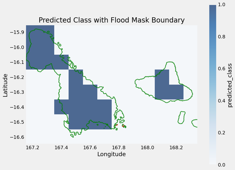
)We can visualize the ground truth flood regions from the ground truth mask. Note that we do capture the general areas impacted by the flood, but ERA5 is a much lower resolution and is masked to land, so some coastal regions and small islands may not contain data in ERA5.
# Extract the mask for pixels with value 2 (flood)
flood_mask_2 = (flood_mask == 2)

# Find indices of those pixels
y_idx, x_idx = np.where(flood_mask_2)

# Get lat/lon for those pixels
lats = flood_mask.y[y_idx].values
lons = flood_mask.x[x_idx].values

# Calculate pixel resolution (assuming regular grid)
res_lat = np.abs(flood_mask.y[1] - flood_mask.y[0]).item()
res_lon = np.abs(flood_mask.x[1] - flood_mask.x[0]).item()

# Build polygons for each pixel
geoms = [
    box(lon - res_lon/2, lat - res_lat/2, lon + res_lon/2, lat + res_lat/2)
    for lon, lat in zip(lons, lats)
]

# Merge polygons into one boundary
merged_geom = unary_union(geoms)
flood_boundary_gdf = gpd.GeoDataFrame(geometry=[merged_geom], crs="EPSG:4326")

# Plot raster prediction using matplotlib
fig, ax = plt.subplots(figsize=(10, 8))
full_pred_ds["predicted_class"].isel(valid_time=0).plot(ax=ax, cmap="Blues", alpha=0.7)

malampa_gdf.boundary.plot(ax=ax, edgecolor='green', linewidth=2, alpha=0.8, label='Malampa Boundary')

# Plot the flood boundary polygon on top in red
flood_boundary_gdf.boundary.plot(ax=ax, edgecolor='red', linewidth=2, alpha=0.7)


plt.title("Predicted Class with Flood Mask Boundary")
plt.xlabel("Longitude")
plt.ylabel("Latitude")
plt.show()
- Montesarchio, V., Napolitano, F., Rianna, M., Ridolfi, E., Russo, F., & Sebastianelli, S. (2014). Comparison of methodologies for flood rainfall thresholds estimation. Natural Hazards, 75(1), 909–934. 10.1007/s11069-014-1357-3
- Yu, T., Ran, Q., Pan, H., Li, J., Pan, J., & Ye, S. (2023). The impacts of rainfall and soil moisture to flood hazards in a humid mountainous catchment: a modeling investigation. Frontiers in Earth Science, 11. 10.3389/feart.2023.1285766
- Yu, T., Ran, Q., Pan, H., Li, J., Pan, J., & Ye, S. (2023). The impacts of rainfall and soil moisture to flood hazards in a humid mountainous catchment: a modeling investigation. Frontiers in Earth Science, 11. 10.3389/feart.2023.1285766