Marine heat wave future projections
This notebook is for forecasting future marine heat wave (MHW) trends.
For a live MHW tracked, check out https://
In this tutorial, we’ll cover the following:
Select CMIP6
tosproduct based on SSP scenarioLoad sea surface temperature (
tos) climate variableCalculate marine heat wave climate indice based on multi-variate data
References:
# !mamba uninstall -y odc-loader
# !mamba install -y cartopy obstore 'zarr>=3' 'python=3.11'
import cartopy.crs as ccrs
import dask.diagnostics
import matplotlib.pyplot as plt
import obstore
import pandas as pd
import xarray as xr
import xclim
import zarrPart 1: Getting cloud hosted CMIP6 data
The Coupled Model Intercomparison Project Phase 6 (CMIP6) dataset is a rich archive of modelling experiments carried out to predict the climate change impacts. The datasets are stored using the Zarr format, and we’ll go over how to access it.
Note: This section was adapted from https://
Sources:
CMIP6 data hosted on Google Cloud - https://
console .cloud .google .com /marketplace /details /noaa -public /cmip6 Pangeo/ESGF Cloud Data Access tutorial - https://
pangeo -data .github .io /pangeo -cmip6 -cloud /accessing _data .html
df = pd.read_csv("https://cmip6.storage.googleapis.com/pangeo-cmip6.csv")
print(f"Number of rows: {len(df)}")
Number of rows: 514818
Over 500,000 rows! Let’s filter it down to the variable and experiment we’re interested in, e.g. sea surface temperature.
For the variable_id, you can look it up given some keyword at
https://
For the table_id, we will filter to just ‘Oday’ for daily measurements.
Another good place to find the right model runs is https://
Below, we’ll filter to CMIP6 experiments matching:
Sea Surface Temperature [degC] (variable_id:
tos)Daily measurements (table_id:
Oday)Model from Geophysical Fluid Dynamics Laboratory’s Coupled Climate Model 4 (source_id:
GFDL-CM4) which is known to have higher resolution ocean models (25km)
References:
Dhage, L., & Widlansky, M. J. (2022). Assessment of 21st Century Changing Sea Surface Temperature, Rainfall, and Sea Surface Height Patterns in the Tropical Pacific Islands Using CMIP6 Greenhouse Warming Projections. Earth’s Future, 10(4), e2021EF002524. Dhage & Widlansky (2022)
Dunne, J. P., Horowitz, L. W., Adcroft, A. J., Ginoux, P., Held, I. M., John, J. G., Krasting, J. P., Malyshev, S., Naik, V., Paulot, F., Shevliakova, E., Stock, C. A., Zadeh, N., Balaji, V., Blanton, C., Dunne, K. A., Dupuis, C., Durachta, J., Dussin, R., … Zhao, M. (2020). The GFDL Earth System Model Version 4.1 (GFDL‐ESM 4.1): Overall Coupled Model Description and Simulation Characteristics. Journal of Advances in Modeling Earth Systems, 12(11), e2019MS002015. Dunne et al. (2020)
df_tos = df.query("variable_id == 'tos' & table_id == 'Oday' & source_id == 'GFDL-CM4'") #
df_tosPart 2: Choose SSP scenario and read from Zarr store
Now to choose a shared socio-economic pathway (SSP) scenario. These are the possible choices for future projections:
‘ssp245’
‘ssp585’
# Shared Socio-economic pathway
SSP_ID = "ssp585"
store_url = df_tos.query(f"experiment_id == '{SSP_ID}'").zstore.iloc[-1]
print(store_url)gs://cmip6/CMIP6/ScenarioMIP/NOAA-GFDL/GFDL-CM4/ssp585/r1i1p1f1/Oday/tos/gr/v20180701/
In many cases, you’ll need to first connect to the cloud provider. The CMIP6 dataset allows anonymous access, but for some cases, you may need to authentication.
We’ll connect to the CMIP6 Zarr store on Google Cloud using
zarr.storage.ObjectStore:
gcs_store = obstore.store.from_url(url=store_url, skip_signature=True)
store = zarr.storage.ObjectStore(store=gcs_store, read_only=True)
Once the Zarr store connection is in place, we can open it into an xarray.Dataset like so.
ds = xr.open_zarr(store=store, consolidated=True, zarr_format=2)
ds
/srv/conda/envs/notebook/lib/python3.11/site-packages/xarray_sentinel/esa_safe.py:7: UserWarning: pkg_resources is deprecated as an API. See https://setuptools.pypa.io/en/latest/pkg_resources.html. The pkg_resources package is slated for removal as early as 2025-11-30. Refrain from using this package or pin to Setuptools<81.
import pkg_resources
ds_vanuatu = ds.sel(lon=slice(166, 170), lat=slice(-22, -11))
ds_vanuatuPart 3: Compute climate indicators using xclim
The xclim library allows us to compute climate indicators based on
some statistic from raw climate values such as temperature or precipitation.
There is no built-in function for marine heat waves yet (see
Ouranosinc
Marine heatwaves (MHWs) are defined as ‘discrete, prolonged anomalously warm water events which last for five or more days, with sea surface temperatures (SSTs) warmer than the 90th percentile relative to climatological values’.
Let’s first calculate the climatological 90th percentile sea surface temperature for the 2020-2050 time period.
tos90_2035 = xclim.core.calendar.percentile_doy(
    arr=ds_vanuatu.sel(time=slice("2020", "2050")).tos,
    window=5,
    per=90,
)
tos90_2035Once that’s done, we can calculate the Warm spell duration index in a calendar year.
da_mhw = xclim.indicators.atmos.warm_spell_duration_index(
    tasmax=ds_vanuatu.tos,  # manually change air temperature to sea surface temperature
    tasmax_per=tos90_2035.sel(percentiles=90).unify_chunks(),
    window=5,
)
da_mhw
/srv/conda/envs/notebook/lib/python3.11/site-packages/xclim/core/cfchecks.py:77: UserWarning: Variable has a non-conforming cell_methods: Got `area: mean where sea time: mean`, which do not include the expected `time: maximum`.
_check_cell_methods(getattr(vardata, "cell_methods", None), data["cell_methods"])
/srv/conda/envs/notebook/lib/python3.11/site-packages/xclim/core/cfchecks.py:79: UserWarning: Variable has a non-conforming standard_name: Got `sea_surface_temperature`, expected `['air_temperature']`
check_valid(vardata, "standard_name", data["standard_name"])
We have 1 model, over 86 timesteps (2015-2100), across 19x4 pixels over Vanuatu. Let’s compute this ‘marine heat wave’ indicator for one year only.
We can also compute this ‘marine heat wave’ indicator for 2050.
Note: Unfortunately, it will take too long to compute this indicator for a full time-series from 2025-2100, so we’ll just pick select years.
with dask.diagnostics.ProgressBar():
    vu_mhw_2050 = da_mhw.sel(time="2050").isel(time=0).compute()
[########################################] | 100% Completed | 36.78 s
projection = ccrs.epsg(code=3832)  # PDC Mercator
fig, ax = plt.subplots(nrows=1, ncols=1, subplot_kw=dict(projection=projection))
vu_mhw_2050.sel(lon=slice(166, 170), lat=slice(-22, -11)).plot.imshow(
    ax=ax, transform=ccrs.PlateCarree()
)
ax.set_extent(extents=[166, 170, -22, -11], crs=ccrs.PlateCarree())
ax.coastlines()
<cartopy.mpl.feature_artist.FeatureArtist at 0x7f12e16d0b10>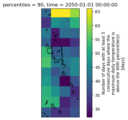
Do the results match with the report from https://www.vanclimatefutures.gov.vu/assets/docs/Marine Heat Waves.pdf ?
Under the high emissions scenario (SSP585) this [Marine Heat Wave] increases to about 170–310 days per year by 2050, with many days in the ‘Strong’ and ‘Severe’ MHW categories
How about for the end of the century (2100)? We’ll need to calculate a different climatology, and then calculate the warm spell duration for that.
tos90_2085 = xclim.core.calendar.percentile_doy(
    arr=ds_vanuatu.sel(time=slice("2070", "2100")).tos,
    window=5,
    per=90,
)
tos90_2085da_mhw = xclim.indicators.atmos.warm_spell_duration_index(
tasmax=ds_vanuatu.tos, # manually change air temperature to sea surface temperature
tasmax_per=tos90_2085.sel(percentiles=90).unify_chunks(),
window=5,
)
da_mhw/srv/conda/envs/notebook/lib/python3.11/site-packages/xclim/core/cfchecks.py:77: UserWarning: Variable has a non-conforming cell_methods: Got `area: mean where sea time: mean`, which do not include the expected `time: maximum`.
_check_cell_methods(getattr(vardata, "cell_methods", None), data["cell_methods"])
/srv/conda/envs/notebook/lib/python3.11/site-packages/xclim/core/cfchecks.py:79: UserWarning: Variable has a non-conforming standard_name: Got `sea_surface_temperature`, expected `['air_temperature']`
check_valid(vardata, "standard_name", data["standard_name"])
with dask.diagnostics.ProgressBar():
    vu_mhw_2100 = da_mhw.sel(time="2100").isel(time=0).compute()
[########################################] | 100% Completed | 37.54 s
projection = ccrs.epsg(code=3832)  # PDC Mercator
fig, ax = plt.subplots(nrows=1, ncols=1, subplot_kw=dict(projection=projection))
vu_mhw_2100.sel(lon=slice(166, 170), lat=slice(-22, -11)).plot.imshow(
    ax=ax, transform=ccrs.PlateCarree()
)
ax.set_extent(extents=[166, 170, -22, -11], crs=ccrs.PlateCarree())
ax.coastlines()
<cartopy.mpl.feature_artist.FeatureArtist at 0x7f1266b43290>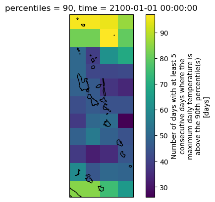
That’s all! Hopefully this will get you started on how to handle CMIP6 climate data for forecasting marine heat waves.
- Dhage, L., & Widlansky, M. J. (2022). Assessment of 21st Century Changing Sea Surface Temperature, Rainfall, and Sea Surface Height Patterns in the Tropical Pacific Islands Using CMIP6 Greenhouse Warming Projections. Earth’s Future, 10(4). 10.1029/2021ef002524
- Dunne, J. P., Horowitz, L. W., Adcroft, A. J., Ginoux, P., Held, I. M., John, J. G., Krasting, J. P., Malyshev, S., Naik, V., Paulot, F., Shevliakova, E., Stock, C. A., Zadeh, N., Balaji, V., Blanton, C., Dunne, K. A., Dupuis, C., Durachta, J., Dussin, R., … Zhao, M. (2020). The GFDL Earth System Model Version 4.1 (GFDL‐ESM 4.1): Overall Coupled Model Description and Simulation Characteristics. Journal of Advances in Modeling Earth Systems, 12(11). 10.1029/2019ms002015