In this lesson, we’ll be looking at coastal erosion (retreat) and accretion (growth) over time in Vanuatu, based on DEP’s Pacific Coastlines (Beta) product. This product consists of annual shorelines at mean sea level, created by combining Landsat collection 2 surface reflectance data with tidal modelling (Bishop-Taylor et al., 2021). It also comes with a rates of change point dataset that provides coastal change statistics at every 30 metres along shorelines.
Links:
DEP map interface: https://
maps .digitalearthpacific .org / #share = s -tIricadkEWrHOQy58RD1 Data download: https://
data .digitalearthpacific .org / #dep _ls _coastlines/ Tileserver endpoint (WMTS, XYZ, etc): https://
tileserver .prod .digitalearthpacific .io/
References:
Bishop-Taylor, R., Nanson, R., Sagar, S., Lymburner, L. (2021). Mapping Australia’s dynamic coastline at mean sea level using three decades of Landsat imagery. Remote Sensing of Environment, 267, 112734. Available: Bishop-Taylor et al. (2021).
https://
knowledge .dea .ga .gov .au /notebooks /Real _world _examples /Coastal _erosion/
# !mamba install -y obstoreimport os
import urllib.request
import geopandas as gpd
import obstore
import pyproj
import shapely.geometryData filtering
The DEP Coastline (v0.7.0.55, released July 2025) covers the entire Pacific and comes in a geopackage file. The 1.97 GB file can be downloaded from:
https://
s3 .us -west -2 .amazonaws .com /dep -public -data /dep _ls _coastlines /dep _ls _coastlines _0 -7 -0 -55 .gpkg
The geopackage file contains several layers. We will be using just two today:
shorelines_annual(line): represents the median shoreline (edge-of-water) location at approximately mean sea level for each year.rates_of_change(point): provides rates of coastal change (in metres per year) at every 30 m along shorelines. These rates are calculated by performing a linear regression between annual shoreline positions and time (year), using the most recent shoreline as the baseline
Let’s stream the file using obstore, and read the shorelines_annual layer into a
geopandas.GeoDataFrame.
We will set a filter to just Vanuatu (VUT)'s Exclusive Economic Zone (EEZ).
# if not os.path.exists("dep_ls_coastlines_0-7-0-55.gpkg"):
#     urllib.request.urlretrieve(
#         url="https://s3.us-west-2.amazonaws.com/dep-public-data/dep_ls_coastlines/dep_ls_coastlines_0-7-0-55.gpkg",
#         filename="dep_ls_coastlines_0-7-0-55.gpkg",
#     )
store = obstore.store.from_url(url="https://s3.us-west-2.amazonaws.com/dep-public-data")
response = obstore.get(
store=store, path="dep_ls_coastlines/dep_ls_coastlines_0-7-0-55.gpkg"
)
byte_stream = response.bytes().to_bytes()gdf_shorelines = gpd.read_file(
# filename="dep_ls_coastlines_0-7-0-55.gpkg",
filename=byte_stream,
layer="shorelines_annual",
where="eez_territory == 'VUT'", # SQL filter to just Vanuatu
)
gdf_shorelines/srv/conda/envs/notebook/lib/python3.10/site-packages/pyogrio/raw.py:198: RuntimeWarning: File /vsimem/pyogrio_3dde6bdd65a34378b34ab27fba3a76ff has GPKG application_id, but non conformant file extension
return ogr_read(
The annual_shoreline data consists of the following columns:
year: The year represented by the corresponding shorelinecertainty: “good” to indicate high quality data, “insufficient data” to indicate that not enough data was available for that year to ensure high quality output, or “unstable data” to indicate the data was highly variable within that yeareez_territory: A 3-letter country code to indicate the economic exclusion zone within which the shoreline fallsgeometry: MultiLineString geometry for the corresponding row.
Next, let’s read the rates_of_change layer, also filtering to just VUT,
plus an additional condition to choose only certainty == 'good' points.
gdf_ratesofchange = gpd.read_file(
    # filename="dep_ls_coastlines_0-7-0-55.gpkg",
    filename=byte_stream,
    layer="rates_of_change",
    where="eez_territory == 'VUT' AND certainty == 'good'",  # SQL filter to Vanuatu & good quality points only
)
print(f"Total: {len(gdf_ratesofchange)} rows")
gdf_ratesofchange.head(n=3)
/srv/conda/envs/notebook/lib/python3.10/site-packages/pyogrio/raw.py:198: RuntimeWarning: File /vsimem/pyogrio_2bfc7d8f63a04d4b97f2fb50c3d6bd3e has GPKG application_id, but non conformant file extension
return ogr_read(
Total: 24053 rows
The rates_of_change data consists of the following columns:
rate_time: Annual rates of change (in metres per year) calculated by linearly regressing annual shoreline distances against time (excluding outliers). Negative values indicate retreat and positive values indicate growthsig_time: Significance (p-value) of the linear relationship between annual shoreline distances and time. Small values (e.g. p-value < 0.01) may indicate a coastline is undergoing consistent coastal change through time.se_time: Standard error (in metres) of the linear relationship between annual shoreline distances and time. This can be used to generate confidence intervals around the rate of change given by rate_time (e.g. 95% confidence interval = se_time * 1.96).outl_time: Individual annual shorelines are noisy estimators of coastline position that can be influenced by environmental conditions (e.g. clouds, breaking waves, sea spray) or modelling issues (e.g. poor tidal modelling results or limited clear satellite observations). To obtain reliable rates of change, outlier shorelines are excluded using a robust Median Absolute Deviation outlier detection algorithm, and recorded in this column.sce: Shoreline Change Envelope (SCE). A measure of the maximum change or variability across all annual shorelines, calculated by computing the maximum distance between any two annual shoreline (excluding outliers). This statistic excludes sub-annual shoreline variability.nsm: Net Shoreline Movement (NSM). The distance between the oldest and most recent annual shoreline (excluding outliers). Negative values indicate the coastline retreated between the oldest and most recent shoreline; positive values indicate growth. This statistic does not reflect sub-annual shoreline variability, so will underestimate the full extent of variability at any given location.max_year,min_year: The year that annual shorelines were at their maximum (i.e. located furthest towards the ocean) and their minimum (i.e. located furthest inland) respectively (excluding outliers). This statistic excludes sub-annual shoreline variability.dist_<year>: The distance between the shoreline position in the last year (2024) and the indicated year. Positive values indicate seaward movement of shorelines, negative values landward.certainty: “good” to indicate high quality data, “insufficient observations” to indicate less than 15 years of observations were available, “extreme value” to indicate the rates of change are greater than 200-m / year, and “high angular variability” to indicate the standard deviation of the angle between the last year and other years is >30 degrees.
Analysis
We now have coastline data for the whole of Vanuatu. Let’s zoom into one small island as a case study.
# Longitude/latitude extend of AOI (Lathu, north of Hog Harbour / Lonnoc Beach)
lonmin = 167.116
lonmax = 167.141
latmin = -15.113
latmax = -15.097
bbox_lonlat = shapely.geometry.box(minx=lonmin, miny=latmin, maxx=lonmax, maxy=latmax)

# Reproject from lon/lat to EPSG:3832
proj_func = pyproj.Transformer.from_crs(
    crs_from="OGC:CRS84", crs_to="EPSG:3832", always_xy=True
).transform
bbox_3832 = shapely.ops.transform(func=proj_func, geom=bbox_lonlat)
bbox_3832xmin, ymin, xmax, ymax = bbox_3832.bounds
gdf_shorelines_crop = gdf_shorelines.clip(mask=bbox_3832)
gdf_ratesofchange_crop = gdf_ratesofchange.clip(mask=bbox_3832)gdf_shorelines_crop.plot(column="year", cmap="viridis", legend=True)<Axes: >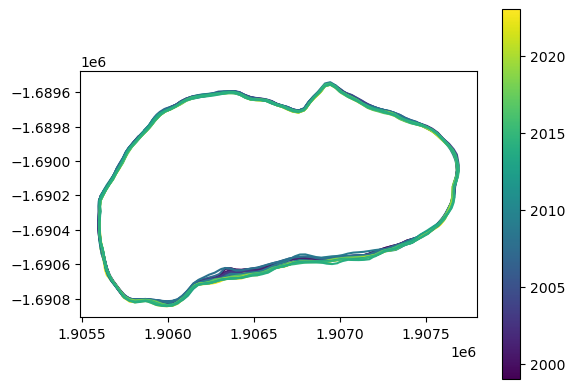
gdf_ratesofchange_crop.plot(
    column="rate_time", cmap="managua", vmin=-2, vmax=2, legend=True
)
<Axes: >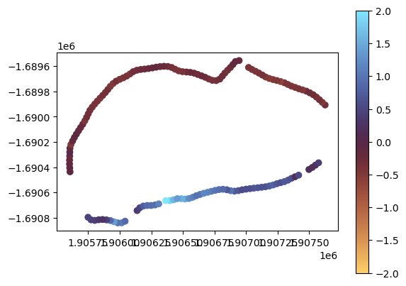
Here, we can see that the Northern shoreline of the island is retreating, whereas the Southern part of the island is expanding.
Export for whole country
Let’s now save the Vanuatu coastlines data to a geopackage (GPKG) file, which can hold
both the shorelines_annual and rates_of_change layers, plus QGIS styles.
# Save annual shorelines
gdf_shorelines.to_file(
    filename="dep_ls_coastlines_vut_0-7-0-55.gpkg",
    layer="shorelines_annual",
    driver="GPKG",
    mode="w",
)
# Save rates of change
gdf_ratesofchange.to_file(
filename="dep_ls_coastlines_vut_0-7-0-55.gpkg",
layer="rates_of_change",
driver="GPKG",
)# Save QGIS styles
gdf_styles = gpd.read_file(
# filename="dep_ls_coastlines_0-7-0-55.gpkg",
filename=byte_stream,
layer="layer_styles",
)
gdf_styles.to_file(
filename="dep_ls_coastlines_vut_0-7-0-55.gpkg",
layer="layer_styles",
driver="GPKG",
)- Bishop-Taylor, R., Nanson, R., Sagar, S., & Lymburner, L. (2021). Mapping Australia’s dynamic coastline at mean sea level using three decades of Landsat imagery. Remote Sensing of Environment, 267, 112734. 10.1016/j.rse.2021.112734