Road segmentation - ML training for Climate Change and Natural Disasters

In this notebook, we’ll be segmenting road networks from aerial imagery.

At the end, you will have trained a model to predict road segments over Port Vila.

Map showing RGB image, predicted roads, and groundtruth road masks over Port Vila.

!pip install -q torch xbatcher segmentation-models-pytorch

import geocube.api.core
import geopandas as gpd
import matplotlib.pyplot as plt
import rioxarray
import segmentation_models_pytorch as smp
import torch
import tqdm
import xarray as xr
import xbatcher.loaders.torch

Data preprocessing¶

Get image data from OpenAerialMap¶

OpenAerialMap images over Vanuatu - https://map.openaerialmap.org/#/168.3819580078125,-16.688816956180833,7

We’ll be using a Maxar Worldview-2 image with a spatial resolution of 32cm over Port Vila on 2024 October 19.

Preview at https://map.openaerialmap.org/#/168.31419467926025,-17.73086527059167,14/square/311123113/676737799f511a0001cc98c1

image_url = "https://oin-hotosm-temp.s3.us-east-1.amazonaws.com/676733089f511a0001cc98b6/0/676733089f511a0001cc98b7.tif"

The RGB images are distributed in a Cloud-optimized GeoTIFF (COG) format. We’ll follow https://corteva.github.io/rioxarray/stable/examples/COG.html to open the file in Python.

Note: We set overview_level=2 to get a lower resolution image. The spatial resolutions at different overview levels are:

Level -1 (native): 0.32 meters
Level 0: 0.64 meters
Level 1: 1.28 meters
Level 2: 2.57 meters

rda = rioxarray.open_rasterio(filename=image_url, overview_level=2)
rda

# Check spatial resolution in meters
rda.rio.resolution()

# Check coordinate reference system
rda.rio.crs.to_string()

# Check bounding box extent
bbox = rda.rio.bounds()
bbox

The image in an xarray.DataArray can be plotted using .plot.imshow(rgb="band")

rda.plot.imshow(rgb="band")

There are some black NoData/NaN areas, let’s crop them out using .rio.clip_box.

rda_portvila = rda.rio.clip_box(
    minx=18732000, miny=-2012000, maxx=18742000, maxy=-2002000
)

rda_portvila.plot.imshow(rgb="band")

bbox_portvila = rda_portvila.rio.bounds()
bbox_portvila

Load road linestrings from shapefile¶

Read from zipfile containing “Roads_Vanuatu_Cleaned_UNOSAT.shp” into a geopandas.GeoDataFrame.

gdf_roads = gpd.read_file(filename="Roads_VUT.zip")
gdf_roads.head()

Reproject vector roads to match aerial image¶

The vector road shapefile are in EPSG:4326, and we will need to reproject it to EPSG:3857 to match the RGB image.

gdf_roads_3857 = gdf_roads.to_crs(crs="EPSG:3857")

Next, we’ll also clip the roads to the bounding box extent of the RGB image.

gdf_roads_portvila = gdf_roads_3857.clip(mask=bbox_portvila)

Plot the clipped vector roads using .plot()

gdf_roads_portvila.plot()

Rasterize road lines¶

The vector road lines need to be converted into a raster format for the machine learning model. We’ll first buffer the road lines to become polygons, and then rasterize them using geocube.api.core.make_geocube.

# Assume all roads are 8 meters in width
gdf_roads_portvila.geometry = gdf_roads_portvila.buffer(distance=8)

rds_roads = geocube.api.core.make_geocube(
    vector_data=gdf_roads_portvila,
    like=rda_portvila,
    measurements=["FID_Road_w"],
)

# Convert to binary where 0=no_roads, 1=roads
rda_roads = rds_roads.FID_Road_w.notnull()

rda_roads.plot.imshow()

Stack RGB image and road mask together¶

We now have an RGB aerial image and rasterized Road map, both in an xarray.DataArray format with the same spatial resolution and bounding box spatial extent. Let’s stack them together using xarray.merge.

ds_image_and_mask = xr.merge(
    objects=[rda_portvila.rename("image"), rda_roads.rename("mask")],
    join="override",
)
ds_image_and_mask

Double check to see that resulting xarray.Dataset’s image and mask looks ok.

# Create subplot with RGB image on the left and Road mask on the right
fig, axs = plt.subplots(ncols=2, figsize=(11.5, 4.5), sharey=True)
ds_image_and_mask.image.plot.imshow(ax=axs[0], rgb="band")
axs[0].set_title("Maxar RGB image")
ds_image_and_mask.mask.plot.imshow(ax=axs[1], cmap="Blues")
axs[1].set_title("Road mask")
plt.show()

Dataloader and Model architecture¶

Now let’s set up our torch DataLoader and a UNet model!

Create data chips with xbatcher¶

The entire image size (~3800x3800 pixels) is too large to fit in memory, so let’s create 256x256 pixel chips using a library called xbatcher that will also help us create a torch Dataset and DataLoader in a few lines of code.

References:

https://xbatcher.readthedocs.io/en/latest/user-guide/training-a-neural-network-with-Pytorch-and-xbatcher.html#Step-2:-Create-batch-generator-and-data-loader

# Define batch generators
X_bgen = xbatcher.BatchGenerator(
    ds_image_and_mask["image"], input_dims={"y": 256, "x": 256}
)
y_bgen = xbatcher.BatchGenerator(
    ds_image_and_mask["mask"], input_dims={"y": 256, "x": 256}
)

# Map batches to a PyTorch-compatible dataset
dataset = xbatcher.loaders.torch.MapDataset(X_generator=X_bgen, y_generator=y_bgen)
# Create a dataloader
dataloader = torch.utils.data.DataLoader(dataset=dataset, batch_size=32)

UNet Model¶

For simplicity, we’ll use a pre-designed model architecture from https://pytorch.org/hub/mateuszbuda_brain-segmentation-pytorch_unet

model = torch.hub.load(
    repo_or_dir="mateuszbuda/brain-segmentation-pytorch",
    model="unet",
    trust_repo=True,
    in_channels=3,
    out_channels=1,
    init_features=32,
    pretrained=True,
)
if torch.cuda.is_available():
    model = model.to(device="cuda")

model

Train the neural network¶

Now is the time to train the UNet model! We’ll need to:

Choose a loss function and optimizer. Here we’re using a DiceLoss with the Adam optimizer.
Configure training hyperparameters such as the learning rate (lr) and number of epochs (max_epochs) or iterations over the entire training dataset.
Construct the main training loop to:
- get a mini-batch from the DataLoader
- pass the mini-batch data into the model to get a prediction
- minimize the error (or loss) between the prediction and groundtruth

Let’s see how this is done!

# Setup loss function and optimizer
loss_dice = smp.losses.DiceLoss(mode="binary")
optimizer = torch.optim.Adam(params=model.parameters(), lr=0.001)

# Main training loop
max_epochs: int = 10
size = len(dataloader.dataset)
for epoch in tqdm.tqdm(iterable=range(max_epochs)):
    for i, batch in enumerate(dataloader):
        # Split data into input (x) and target (y)
        image, mask = batch
        # assert image.shape == (2, 3, 128, 128), image.shape
        # assert mask.shape == (2, 128, 128), mask.shape
        assert image.device == torch.device("cpu")  # Data is on CPU

        # Move data to GPU if available
        if torch.cuda.is_available():
            image = image.to(device="cuda")  # Move data to GPU
            assert image.device == torch.device("cuda:0")  # Data is on GPU now!
            mask = mask.to(device="cuda")

        # Pass data into neural network model
        prediction = model(x=image.float())

        # Compute prediction error
        loss = loss_dice(
            y_pred=prediction.squeeze(dim=1), y_true=mask.to(dtype=torch.float32)
        )

        # Backpropagation (to minimize loss)
        loss.backward()
        optimizer.step()
        optimizer.zero_grad()

        # Report metrics
        current = (i + 1) * len(image)
        print(f"loss: {loss:>7f}  [{current:>5d}/{size:>5d}]")

Inference results¶

Besides monitoring the loss value, it is also good to calculate a metric like Precision, Recall or F1-score. Let’s first run the model in ‘inference’ mode to get predictions.

index = 21  # TODO change this to check a different image
image, mask = dataloader.dataset[index]
with torch.inference_mode():
    pred = model(x=image.unsqueeze(dim=0).to(device="cuda").float())
    pred = pred.cpu().squeeze(dim=(0, 1))

Now that we have the predicted road image, we can compute some metrics.

# compute statistics for true positive, false positive, false negative and true negative "pixels"
tp, fp, fn, tn = smp.metrics.get_stats(
    output=pred, target=mask, mode="binary", threshold=0.5
)
f1_score = smp.metrics.f1_score(tp=tp, fp=fp, fn=fn, tn=tn, reduction="micro")
precision = smp.metrics.precision(
    tp=tp, fp=fp, fn=fn, tn=tn, reduction="micro-imagewise"
)
recall = smp.metrics.recall(tp=tp, fp=fp, fn=fn, tn=tn, reduction="micro-imagewise")
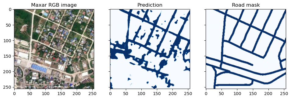
print(f"F1 Score: {f1_score:.4f}, Precision: {precision:.4f}, Recall: {recall:.4f}")

Finally, let’s compare the model predicted road to the ‘groundtruth’ road mask by visualizing it side by side as below.

# Create subplot with RGB image on the left, prediction in middle, and Road mask on the right
fig, axs = plt.subplots(ncols=3, figsize=(11.5, 4.5), sharey=True)
axs[0].imshow(image.permute(1, 2, 0))
axs[0].set_title("Maxar RGB image")
axs[1].imshow(pred, cmap="Blues", vmin=0, vmax=1)
axs[1].set_title("Prediction")
axs[2].imshow(mask, cmap="Blues")
axs[2].set_title("Road mask")
plt.show()

Let’s save the RGB image and output prediction to a GeoTIFF file.

coords_image = dataloader.dataset.X_generator[index].coords
rgb_image = xr.DataArray(data=image, coords=coords_image)
rgb_image.rio.to_raster(raster_path="rgb_image.tif", driver="COG")

coords_roads = dataloader.dataset.y_generator[index].coords
pred_roads = xr.DataArray(data=pred, coords=coords_roads)
pred_roads.rio.to_raster(raster_path="predicted_roads.tif", driver="COG")

You can now download the *.tif files from the left sidebar, and put them into a desktop GIS to view. It is also possible to convert the predicted raster roads into a vector polygon using QGIS’s Raster -> Conversion -> Polygonize function that is based on the gdal_polygonize program.