Data Acquisition:
Downloading the Tropical and Sub-Tropical Flood and Water Masks dataset.
Fetching Sentinel-1 RTC (for SAR-based flood detection) from STAC for Vanuatu and the relevant surrounding region.
Preprocessing:
Aligning Sentinel-1 data.
Normalization, filtering, and masking.
Preparing training data by pairing inputs (SAR images) with water masks.
Model Definition:
Implementing a U-Net (CNN) in PyTorch for segmentation.
Training & Evaluation:
Splitting data into train/val/test sets.
Data loading through batches.
Loss function and optimizer.
Model training loop.
Performance evaluation with IoU and Accuracy Score.
Inference & Visualization:
Running the model on test images.
Plotting predicted masks.
This sets up a basic segmentation pipeline using U-Net and PyTorch, processing Sentinel-1 data for flood and water masks.
!pip install -q torch torchvision gdownimport os
import glob
import math
from datetime import datetime, timedelta
import torch
import torch.nn as nn
import torch.nn.functional as F
import torch.optim as optim
from torch.utils.data import DataLoader, Dataset, random_split
import torchvision.transforms as transforms
import torchvision
import pandas as pd
import numpy as np
import geopandas as gpd
import rasterio
from rasterio.features import shapes
import tqdm
import xarray as xr
import rioxarray as rxr
import planetary_computer
import pystac_client
import odc.stac
import matplotlib.pyplot as plt
import matplotlib.colors as mcolors
from shapely.geometry import box, shape
from sklearn.metrics import jaccard_score, accuracy_score
from skimage.transform import resize
import dask
import dask.array as da
import dask.delayedThe Tropical and Sub-Tropical Flood and Water Masks dataset provides 10-meter spatial resolution masks designed for developing machine learning models to classify flooding in satellite imagery. It comprises 513 GeoTIFF files, each corresponding to specific flood events and dates, covering 65 flood events since 2018 across 26 countries in tropical and sub-tropical regions.
Dataset Composition:
Classes:
0: No data1: Land (not flooded)2: Flooded areas3: Permanent water bodies
Associated Dates:
Activation Date: Date when the flood event was registered in the EMS Rapid Mapping system.
Event Date: Initial date of the flood occurrence.
Satellite Date: Date of the latest satellite imagery used for generating the flood mask.
The masks were generated by integrating data from the ESA WorldCover 10m v100 product and vector layers from the Copernicus Emergency Management System (EMS) Rapid Mapping Activation events.
This dataset is particularly useful for training flood detection models to identify and segment flooded areas in satellite images, and we’ll use it in the specific geographic context of the Pacific region.
The dataset is licensed under the Creative Commons Attribution-NonCommercial 4.0 License.
We’ll obtain the data band then unzip the folder. The labels will be in a subfolder called ‘tst-ground-truth-flood-masks’ and accompanied by a metadata file which we will use for filtering and image acquisition.
# Download the data (subset_vbos_smaller.zip)
!gdown "https://drive.google.com/uc?id=1rLNwGQf8C93CXpdQ293zKaKiQejDdJnp"
# Unzip the compressed data
!mkdir -p vbos/flood/
!unzip subset_vbos_smaller.zip -d vbos/flood/# Get list of all labels
mask_paths = glob.glob('vbos/flood/subset_vbos_smaller/tst-ground-truth-flood-masks/*.tif')len(mask_paths)34ls vbos/flood/subset_vbos_smaller/tst-ground-truth-flood-masks/ | headEMSR269_02FAHEFA_GRA_v1_ground_truth.tif
EMSR269_06VEITONGO_GRA_MONIT01_v1_ground_truth.tif
EMSR269_06VEITONGO_GRA_v2_ground_truth.tif
EMSR312_02CALAYAN_GRA_v1_ground_truth.tif
EMSR312_05TUGUEGARAO_DEL_MONIT01_v1_ground_truth.tif
EMSR312_05TUGUEGARAO_DEL_v1_ground_truth.tif
EMSR312_06ILAGAN_DEL_MONIT01_v1_ground_truth.tif
EMSR312_06ILAGAN_DEL_v1_ground_truth.tif
EMSR312_07VIGAN_DEL_MONIT01_v1_ground_truth.tif
EMSR312_07VIGAN_DEL_v1_ground_truth.tif
cd vbos/flood/subset_vbos_smaller/Let’s implement a U-Net model with a ResNet34 encoder, adapted for image segmentation tasks. The model takes a two-channel input and outputs a four-class segmentation mask.
This entails our first example of a convolution neural network (CNN).
Model Architecture
Encoder (Feature Extraction)
Uses a pre-trained ResNet34 as a feature extractor.
The first convolution layer is modified to accept two input channels (VV and VH SAR polarizations) instead of three (RGB).
The encoder progressively downsamples the input image while extracting high-level features:
encoder1: Initial convolution layer with batch normalization and ReLU.encoder2→encoder5: ResNet34 convolutional layers, reducing spatial dimensions.
Bottleneck Layer
A 1x1 convolution expands the deepest encoder feature map to 1024 channels.
Acts as the bridge between encoder and decoder.
Decoder (Upsampling with Skip Connections)
The decoder upsamples the feature maps back to the original image resolution.
Uses skip connections to concatenate encoder outputs with corresponding decoder layers.
Each upsampling layer consists of:
Bilinear interpolation
3x3 convolution
ReLU activation
Final Segmentation Output
A 1x1 convolution reduces the output to 4 channels (matching the number of segmentation classes).
Ensures the final output size is 224x224.
Skip Connections and Interpolation Handling
Since downsampling reduces spatial dimensions, skip connection tensors are interpolated to match decoder sizes before concatenation.
F.interpolate()is used to ensure spatial compatibility.
Forward Pass (Data Flow)
Input image (B, 2, 224, 224) → passes through encoder (ResNet34) → generates feature maps. Herein, B stands for batch. That is just a small sample of the dataset provided to the model. We have to break down the dataset and provide in small samples of equal size in order to fit on the available RAM.
Bottleneck layer processes the deepest feature representation.
Decoder upsamples while concatenating interpolated skip connections from the encoder.
Final segmentation mask is generated with shape
(B, 4, 224, 224).
This architecture should do well for flood and water segmentation from Sentinel-1 images, given its ability to retain fine-grained spatial details while leveraging ResNet34’s strong feature extraction.
# Define U-Net model with ResNet34 backbone
class UNetWithResNetEncoder(nn.Module):
    def __init__(self, in_channels=2, out_channels=4):
        super().__init__()

        # Load pre-trained ResNet34 backbone
        resnet = torchvision.models.resnet34(weights=torchvision.models.resnet.ResNet34_Weights.DEFAULT)

        # Modify first convolution to accept 2 channels
        self.encoder1 = nn.Sequential(
            nn.Conv2d(in_channels, 64, kernel_size=7, stride=2, padding=3, bias=False),
            resnet.bn1,
            resnet.relu
        )

        # Encoder layers
        self.encoder2 = resnet.layer1  # (B, 64, H/4, W/4)
        self.encoder3 = resnet.layer2  # (B, 128, H/8, W/8)
        self.encoder4 = resnet.layer3  # (B, 256, H/16, W/16)
        self.encoder5 = resnet.layer4  # (B, 512, H/32, W/32)

        # Bottleneck
        self.bottleneck = nn.Conv2d(512, 1024, kernel_size=3, padding=1)

        # Decoder with skip connections
        self.upconv1 = self._upsample(1024, 512)
        self.upconv2 = self._upsample(512 + 512, 256)  # Add encoder5 skip connection
        self.upconv3 = self._upsample(256 + 256, 128)  # Add encoder4 skip connection
        self.upconv4 = self._upsample(128 + 128, 64)   # Add encoder3 skip connection
        self.upconv5 = self._upsample(64 + 64, 64)     # Add encoder2 skip connection

        # Final segmentation output
        self.final_conv = nn.Conv2d(64, out_channels, kernel_size=1)

    def _upsample(self, in_channels, out_channels):
        """Helper function to create upsampling layers."""
        return nn.Sequential(
            nn.Upsample(scale_factor=2, mode="bilinear", align_corners=True),
            nn.Conv2d(in_channels, out_channels, kernel_size=3, padding=1),
            nn.ReLU(inplace=True)
        )

    def forward(self, x):
        # Encoder path
        enc1 = self.encoder1(x)   # (B, 64, 112, 112)
        enc2 = self.encoder2(enc1) # (B, 64, 56, 56)
        enc3 = self.encoder3(enc2) # (B, 128, 28, 28)
        enc4 = self.encoder4(enc3) # (B, 256, 14, 14)
        enc5 = self.encoder5(enc4) # (B, 512, 7, 7)

        # Bottleneck
        x = self.bottleneck(enc5)  # (B, 1024, 7, 7)
        x = self.upconv1(x)        # (B, 512, 14, 14)

        # Ensure enc5 matches x before concatenation
        enc5 = F.interpolate(enc5, size=x.shape[2:], mode="bilinear", align_corners=True)
        x = torch.cat([x, enc5], dim=1)

        x = self.upconv2(x)  # (B, 256, 28, 28)

        # Ensure enc4 matches x before concatenation
        enc4 = F.interpolate(enc4, size=x.shape[2:], mode="bilinear", align_corners=True)
        x = torch.cat([x, enc4], dim=1)

        x = self.upconv3(x)  # (B, 128, 56, 56)

        # Ensure enc3 matches x before concatenation
        enc3 = F.interpolate(enc3, size=x.shape[2:], mode="bilinear", align_corners=True)
        x = torch.cat([x, enc3], dim=1)

        x = self.upconv4(x)  # (B, 64, 112, 112)

        # Ensure enc2 matches x before concatenation
        enc2 = F.interpolate(enc2, size=x.shape[2:], mode="bilinear", align_corners=True)
        x = torch.cat([x, enc2], dim=1)

        x = self.upconv5(x)  # (B, 64, 224, 224)

        # Ensure final output size is exactly (B, 4, 224, 224)
        x = self.final_conv(x)  # (B, 4, 224, 224)
        x = F.interpolate(x, size=(224, 224), mode="bilinear", align_corners=True)  # Fix output size

        return x
The following functions facilitate fetching Sentinel-1 Radiometrically Terrain Corrected (RTC) imagery from the Microsoft Planetary Computer STAC API, using bounding boxes derived from our raster label data.
fetch_s1_rtc_for_date(bounds, date) fetches Sentinel-1 RTC data for a given date (or up to 3 days later) within the specified bounding box.
How It Works
Connects to the Microsoft Planetary Computer STAC API.
Defines a time window of 3 days starting from the given date.
Searches for available Sentinel-1 RTC data within the bounding box.
Signs STAC items using Planetary Computer authentication.
Loads the first available scene as an xarray dataset.
Inputs
bounds: Bounding box (left, bottom, right, top) specifying the geographic area.date: The target date (YYYY-MM-DD format, string).
Returns
An xarray dataset containing the Sentinel-1 RTC image.
If no data is found, returns None.
match_s1_rtc_to_dataframe(df, mask_path) finds and fetches Sentinel-1 RTC imagery corresponding to a given ground truth mask.
How It Works
Searches for the specified mask file (
mask_path) in the given DataFrame (df).Extracts the satellite image acquisition date.
Converts the date format from DD/MM/YYYY to YYYY-MM-DD.
Reads the bounding box (extent) of the mask using Rasterio.
Calls
fetch_s1_rtc_for_date()with the mask’s bounding box and acquisition date.Returns the matching Sentinel-1 RTC dataset.
Inputs
df: A DataFrame containing mask metadata, including file names and acquisition dates.mask_path: The file name of the ground truth flood mask.
Returns
The corresponding Sentinel-1 RTC image as an xarray dataset.
These functions are designed to fetch Sentinel-1 RTC data needed to match our flood masks.
# Function to fetch Sentinel-1 RTC data matching a given date (or up to 3 days after)
def fetch_s1_rtc_for_date(bounds, crs, date):
    catalog = pystac_client.Client.open("https://planetarycomputer.microsoft.com/api/stac/v1")

    # Define the search time range (3-day + window)
    date = datetime.strptime(date, "%Y-%m-%d")  # Convert to datetime object

    start_date = date.strftime("%Y-%m-%d")
    end_date = (date + timedelta(days=3)).strftime("%Y-%m-%d")

    search = catalog.search(
        collections=["sentinel-1-rtc"],
        bbox=[bounds.left, bounds.bottom, bounds.right, bounds.top],
        datetime=f"{start_date}/{end_date}"
    )

    items = list(search.items())
    if not items:
        return None  # No matching data found

    signed_items = [planetary_computer.sign(item) for item in items]

    # Load the first available scene (or refine selection criteria as needed)
    ds = odc.stac.load(signed_items[:1], bbox=bounds, dtype="float32")
    ds = ds.rio.reproject(dst_crs=crs)  # Reproject to same CRS

    return ds.isel(time=0) #.mean(dim="time") if ds else None  # Take mean if multiple images exist

# Function to find matching Sentinel-1 RTC imagery for each row in DataFrame
def match_s1_rtc_to_dataframe(df, mask_path):
    filtered_row = df.loc[df["File Name"] == mask_path].iloc[0]
    sat_date = filtered_row["Satellite Date"]
    formatted_date = datetime.strptime(sat_date, "%d/%m/%Y").strftime("%Y-%m-%d")


    with rasterio.open(f"tst-ground-truth-flood-masks/{mask_path}_ground_truth.tif") as src:
        bounds = src.bounds  # Get bounding box of the mask
        crs = src.crs  # Coordinate Reference System

    s1_image = fetch_s1_rtc_for_date(bounds, crs, formatted_date)

    return s1_image
Load the metadata file into a dataframe and select labels for Vanuatu and a relevant surrounding region so as to provide sufficient data for model training.
df = pd.read_csv('metadata/metadata.csv')
# Filter for specific countries
selected_countries = {"Vanuatu", "Tonga"} #, "Timor-Leste" , "Philippines", "Viet Nam", "Australia"}
df = df[df["Country"].isin(selected_countries)]

"""
# Limit the number of rows for the Philippines
df_philippines = df[df["Country"] == "Philippines"].head(5)  # Keep only 10 rows
df_other = df[df["Country"] != "Philippines"]  # Keep all other countries

# Concatenate back
df = pd.concat([df_philippines, df_other])

# Reset index
df = df.reset_index(drop=True)
"""

print("len(df):", len(df))
len(df): 4
Now let’s establish a dataset class.
This FloodDataset class is a PyTorch Dataset that loads Sentinel-1 RTC images and corresponding flood masks, tiles them into fixed-size patches, and prepares them for training.
Key inputs:
mask_paths: A list of file names representing flood masks.transform: Optional data transformations (not used here).tile_size: Size of the image and mask patches (default: 224x224).
Step 1: Load mask file names
The dataset uses mask file names from the metadata DataFrame (df).
Step 2: Fetch corresponding Sentinel-1 RTC images using Dask
The function
match_s1_rtc_to_dataframe(df, mask_path)fetches Sentinel-1 RTC data for each flood mask using STAC.Uses Dask Delayed to parallelize the fetching process, reducing I/O overhead.
Step 3: Load masks, get Sentinel-1 images and convert them to tensors
Read the ground truth flood mask from the file.
Get Sentinel-1 data. If Sentinel-1 data is unavailable for a mask in the requested time window, it is skipped.
Convert the Sentinel-1 image to a PyTorch tensor.
Convert the mask to a tensor and reshape to match PyTorch conventions.
Step 4: Tile images and masks into 224x224 patches
_tile_image_and_mask()divides the large images and masks into smaller 224x224 tiles.The resulting tiles are stored in lists.
Tiling Function (_tile_image_and_mask)
Splits images and masks into fixed-size tiles.
Loops through the image and mask with a stride of
tile_size(224 pixels).Ensures that only fully-sized tiles (224x224) are added.
Dataset Methods
__len__(self) Returns the total number of 224x224 tiles.
__getitem__(self, idx) returns the corresponding image-mask pair for training.
class FloodDataset(Dataset):
    def __init__(self, mask_paths, transform=None, tile_size=224):
        #self.mask_paths = filter_masks_within_vanuatu(mask_paths)
        self.mask_paths = list(df["File Name"])
        self.transform = transform
        self.image_list = []
        self.mask_list = []
        self.tile_size = tile_size

        # Use Dask Delayed for parallel fetching
        delayed_images = []
        for mask_path in self.mask_paths:
            s1_image = match_s1_rtc_to_dataframe(df, mask_path)
            delayed_images.append(dask.delayed(s1_image))

        # Compute all Dask delayed tasks at once (efficient batch processing)
        computed_images = dask.compute(*delayed_images)

        self.image_tiles = []
        self.mask_tiles = []

        for i, mask_path in enumerate(self.mask_paths):
            if computed_images[i] is None:
                continue  # Skip if no data was found

            with rasterio.open(f"tst-ground-truth-flood-masks/{mask_path}_ground_truth.tif") as src:
                mask = src.read(1).astype(np.float32)
            try:
                image_tensor = torch.tensor(computed_images[i].to_array().values, dtype=torch.float32)
                mask_tensor = torch.tensor(mask).unsqueeze(0)

                image_tiles, mask_tiles = self._tile_image_and_mask(image_tensor, mask_tensor)
                self.image_tiles.extend(image_tiles)  # Flatten the dataset
                self.mask_tiles.extend(mask_tiles)
            except:
                print("error when creating tensor")
                continue


    def __len__(self):
        return len(self.image_tiles)

    def __getitem__(self, idx):
        return self.image_tiles[idx], self.mask_tiles[idx]

    def _tile_image_and_mask(self, image, mask):
        #Tiles both the image and mask into patches of size (tile_size x tile_size).

        height, width = image.shape[-2:]  # Ensure compatibility with tensor dimensions
        image_tiles = []
        mask_tiles = []

        for i in range(0, height, self.tile_size):
            for j in range(0, width, self.tile_size):
                # Extract tiles
                image_tile = image[..., i:i + self.tile_size, j:j + self.tile_size]
                mask_tile = mask[..., i:i + self.tile_size, j:j + self.tile_size]

                if mask_tile.shape[-2] == self.tile_size and mask_tile.shape[-1] == self.tile_size and image_tile.shape[-2] == self.tile_size and image_tile.shape[-1] == self.tile_size:
                    image_tiles.append(image_tile.clone().detach())
                    mask_tiles.append(mask_tile.clone().detach())

        return image_tiles, mask_tiles
Generate the dataset and split it into train, validation and test datasets.
We are reserving 70% of samples for training, 20% for validation and approximately 10% for testing.
Notice we are providing a transform to normalize image values to the range [0, 1]. This improves model stability and convergence since Sentinel-1 RTC images may have different ranges, therefore we need to ensure consistent input scaling.
full_dataset = FloodDataset(mask_paths=mask_paths,
                             transform=transforms.Compose([transforms.Normalize(0, 1)]), tile_size=224)
# Define split sizes
train_size = int(0.7 * len(full_dataset))
val_size = int(0.20 * len(full_dataset))
test_size = len(full_dataset) - train_size - val_size # Ensures total sums up correctly
# Perform split
generator = torch.Generator().manual_seed(42)
train_dataset, val_dataset, test_dataset = random_split(full_dataset, [train_size, val_size, test_size], generator)
print(f"Dataset sizes -> Train: {len(train_dataset)}, Val: {len(val_dataset)}, Test: {len(test_dataset)}")Dataset sizes -> Train: 33, Val: 9, Test: 6
Let’s initialize PyTorch DataLoaders for training, validation, and testing datasets. DataLoaders efficiently manage data loading, batching, and shuffling.
Key Parameters
train_dataset_,val_dataset,test_dataset:These are FloodDataset instances containing image-mask pairs.
batch_size=2:Each batch contains 2 image-mask pairs.
shuffle=True(Training Only):Randomizes data order for better generalization.
shuffle=False(Validation & Test Sets):Keeps a fixed order for consistent evaluation.
drop_last=True:Drops the last batch if it’s smaller than
batch_sizeto ensure consistent batch sizes.
How it works
train_loader:Feeds randomized batches for training, preventing the model from memorizing patterns.
val_loader:Provides sequential batches for model validation.
test_loader:Loads data for final model testing and performance evaluation.
# Create DataLoaders
train_loader = DataLoader(train_dataset, batch_size=2, shuffle=True, drop_last=True)
val_loader = DataLoader(val_dataset, batch_size=2, shuffle=False, drop_last=True)
test_loader = DataLoader(test_dataset, batch_size=2, shuffle=False, drop_last=True)
Now let’s train our U-Net model. We’ll specify some hyperparamets such as the loss function, optimizer and number of epochs to train for.
1. Model, Loss, and Optimizer Setup
model = UNetWithResNetEncoder()Initializes the U-Net model.
criterion = nn.CrossEntropyLoss()Uses CrossEntropyLoss for multi-class segmentation.
optimizer = optim.Adam(model.parameters(), lr=0.001)Uses the Adam optimizer with a learning rate of
0.001to update the model parameters.
2. Training Loop
The training loop runs for a minimal 20 epochs, ensuring the model learns over multiple iterations nut keeping it small for demonstration purposes.
model.train()sets the model in training mode, enabling dropout and batch normalization.We load a batch of images and masks iteratively from
train_loader.outputs = model(images)performs forward propagation and generates predictions.loss = criterion(outputs, masks)measures how different predictions are from ground truth.Backpropagation and optimization:
loss.backward(): Computes gradients.optimizer.step(): Updates model parameters.
4. Validation Phase
model.eval()switches to evaluation mode, disabling dropout and batch norm updates.torch.no_grad()stops gradient computation to save memory and speed up inference.The validation loop computes loss but does not update model weights.
5. Print Epoch Statistics
Computes average training and validation loss for each epoch.
epochs = 20# Model, Loss, Optimizer
model = UNetWithResNetEncoder()
criterion = nn.CrossEntropyLoss()
optimizer = optim.Adam(model.parameters(), lr=0.001)
print("Starting training")
# Training Loop
for epoch in tqdm.trange(epochs):
model.train() # Ensure the model is in training mode
# Training phase
train_loss = 0.0
for batch in train_loader:
images, masks = batch # Unpack stacked tensors
if isinstance(images, list):
images = torch.cat(images, dim=0) # Ensure 4D tensor (B, C, H, W)
if isinstance(masks, list):
masks = torch.cat(masks, dim=0)
images = torch.stack(images) if isinstance(images, list) else images
masks = torch.stack(masks) if isinstance(masks, list) else masks
masks = masks.squeeze()
masks = masks.long() # Convert masks to LongTensor before computing loss
optimizer.zero_grad()
outputs = model(images) # Forward pass
loss = criterion(outputs, masks)
loss.backward()
optimizer.step()
train_loss += loss.item()
# Average training loss for the epoch
train_loss /= len(train_loader)
# Validation phase
model.eval() # Set the model to evaluation mode
val_loss = 0.0
with torch.no_grad():
for batch in val_loader:
images, masks = batch # Unpack stacked tensors
if isinstance(images, list):
images = torch.cat(images, dim=0)
if isinstance(masks, list):
masks = torch.cat(masks, dim=0)
images = torch.stack(images) if isinstance(images, list) else images
masks = torch.stack(masks) if isinstance(masks, list) else masks
masks = masks.squeeze()
masks = masks.long() # Convert masks to LongTensor
outputs = model(images) # Forward pass
loss = criterion(outputs, masks)
val_loss += loss.item()
# Average validation loss for the epoch
val_loss /= len(val_loader)
print(f"Epoch {epoch+1}, Train Loss: {train_loss:.4f}, Validation Loss: {val_loss:.4f}")Save the model to a file for future use. torch.save(model.state_dict(), final_model_path) saves the model’s learned parameters (weights) to the specified path. The .state_dict() method is used because it only saves the model’s parameters, not the entire model structure, which is a more efficient approach. This means we need to re-instate the model class any time in the future in which we want to run inference for this to be complete.
# Directory to save the model checkpoints
MODEL_SAVE_DIR = '.'
os.makedirs(MODEL_SAVE_DIR, exist_ok=True)

# Save the final model after training
final_model_path = os.path.join(MODEL_SAVE_DIR, f"final_model_{epochs}ep.pth")
torch.save(model.state_dict(), final_model_path)
print(f"Final model saved at {final_model_path}")
Final model saved at model_s1/final_model_20ep_vnu_tvt.pth
Now we’ll define an inference function that is used to make predictions with a trained model.
model.eval():
This sets the model to evaluation mode. In evaluation mode, dropout and batch normalization behave differently than during training. This ensures that the model’s behavior is consistent when making predictions.
with torch.no_grad():
This disables the tracking of gradients, which is unnecessary during inference (i.e., when making predictions). Disabling gradients helps reduce memory usage and speeds up the computation.
output = model(image.unsqueeze(0)):
The
image.unsqueeze(0)adds a batch dimension to the input image. Most models expect a batch of images, so even if there is only one image, it is wrapped in a batch.model(image.unsqueeze(0))runs the image through the trained model to generate an output (logits or raw predictions) for each class.
torch.softmax(output, dim=1):
The softmax function is applied to the output along the class dimension (dimension 1). Softmax normalizes the output values into probabilities, so each pixel in the image will have a probability distribution across all the possible classes.
prediction = prediction.squeeze(0):
This removes the batch dimension (which was added earlier using
unsqueeze(0)), returning the prediction in the shape of a single image, but now with probabilities for each pixel in each class.
prediction = torch.argmax(prediction, dim=0).cpu().numpy():
torch.argmax(prediction, dim=0)selects the class with the highest probability for each pixel (i.e., the predicted class label for each pixel)..cpu().numpy()moves the result to the CPU and converts the PyTorch tensor into a NumPy array, which is easier to handle for further processing or visualization outside of PyTorch.
return prediction:
The function returns the final prediction, which is a NumPy array containing the predicted class labels for each pixel.
# Inference Function
def inference(model, image):
    model.eval()
    with torch.no_grad():
        output = model(image.unsqueeze(0)) # 4 channels of logits
        prediction = torch.softmax(output, dim=1).squeeze(0)  # Softmax across channels
        prediction = torch.argmax(prediction, dim=0).cpu().numpy()  # Get class labels
    return prediction # 1, h, w
Let’s define how to execute the evaluation and visualization processes for the trained model. The two functions evaluate() and visualize_prediction() run the evaluation and visualize the model’s predicitive capabilities. The model’s performance is evaluated on the test set.
evaluate():
model.eval(): Just like before, sets the model to evaluation mode, ensuring no dropout and that batch normalization behaves appropriately.with torch.no_grad(): Disables gradient computation, which is unnecessary during evaluation and reduces memory usage.For each batch of images and corresponding ground truth masks, the model’s predictions are calculated.
torch.argmax(outputs, dim=1): Converts the output from the model (which contains predictions across different classes) into the predicted class labels by selecting the class with the highest score for each pixel.Both the predicted and true mask tensors are flattened into 1D arrays for easier comparison.
jaccard_score: Calculates the Intersection over Union (IoU), a measure of overlap between the predicted and ground truth masks.accuracy_score: Calculates the accuracy of the predicted masks compared to the ground truth.
After evaluating all the batches, we calculate and print the average IoU and accuracy scores across the dataset.
visualize_prediction():
Creates a figure with 3 subplots arranged horizontally (image tile, ground truth, prediction), each having the same size.
vv_image = image[0].cpu().numpy(): Converts the first channel of the input Sentinel-1 image tile to a NumPy array for visualization.Displays the generated plots.
# Evaluation Function
def evaluate(model, data_loader):
    model.eval()
    iou_scores, accuracy_scores = [], []
    with torch.no_grad():
        for images, masks in data_loader:
            outputs = model(images)
            preds = torch.argmax(outputs, dim=1)  # Convert [batch, 4, H, W] → [batch, H, W]
            preds = preds.cpu().numpy().flatten()
            masks = masks.cpu().numpy().flatten()
            iou_scores.append(jaccard_score(masks, preds, average="macro"))
            accuracy_scores.append(accuracy_score(masks, preds))
    print(f"Mean IoU: {np.mean(iou_scores):.4f}, Mean Accuracy: {np.mean(accuracy_scores):.4f}")


# Run Evaluation
evaluate(model, test_loader)
# Define class labels and colormap
class_labels = {
0: "No Data",
1: "Land (not flooded)",
2: "Flooded areas",
3: "Permanent water bodies"
}
# Define discrete colormap
cmap = mcolors.ListedColormap(["black", "green", "blue", "navy"]) # Colors for classes 0-3
bounds = [0, 1, 2, 3, 4] # Boundaries between color levels
norm = mcolors.BoundaryNorm(bounds, cmap.N)
def visualize_prediction(image, mask, prediction):
fig, ax = plt.subplots(1, 3, figsize=(15, 5))
# Convert 2-channel image to single-channel (VV)
vv_image = image[0].cpu().numpy() # Use first channel (VV)
ax[0].imshow(vv_image, cmap="gray") # Display as grayscale
ax[0].set_title("Input Image (VV)")
im1 = ax[1].imshow(mask.squeeze(), cmap=cmap, norm=norm)
ax[1].set_title("Ground Truth")
im2 = ax[2].imshow(prediction, cmap=cmap, norm=norm)
ax[2].set_title("Prediction")
# Create colorbar with class labels
cbar = fig.colorbar(im2, ax=ax.ravel().tolist(), ticks=[0.5, 1.5, 2.5, 3.5], orientation="horizontal")
cbar.ax.set_xticklabels([class_labels[i] for i in range(4)]) # Assign class names
plt.show()
# Test Inference and Visualization
sample_image, sample_mask = test_dataset[0]
predicted_mask = inference(model, sample_image)
visualize_prediction(sample_image, sample_mask, predicted_mask)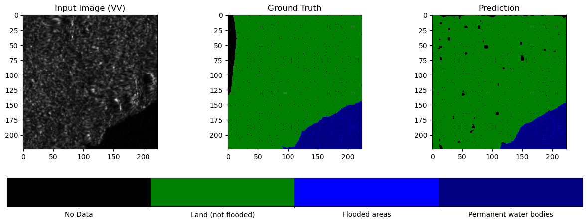
Now let’s use an administrative boundaries file from Pacific Data Hub to get imagery for Vanuatu and run inference on these areas with our trained model.
admin_boundaries_gdf = gpd.read_file("./2016_phc_vut_iid_4326.geojson").to_crs(epsg="4326")admin_boundaries_gdfLoad the saved model from file.
# Define the model architecture (must match the saved model)
model = UNetWithResNetEncoder(in_channels=2, out_channels=4)  # Ensure the same architecture

epochs = 20
# Load the model weights
model.load_state_dict(torch.load(f"final_model_{epochs}ep.pth"))

# Set the model to evaluation mode (important for inference)
model.eval()

#device = torch.device("cuda" if torch.cuda.is_available() else "cpu")
#model.to(device)
New function to get relevant Sentinel-1 imagery within 10 days after the requested date.
# Function to fetch Sentinel-1 RTC data matching a given date (or up to 10 days after)
def fetch_s1_rtc_for_date_inference(bounds, date):
    catalog = pystac_client.Client.open("https://planetarycomputer.microsoft.com/api/stac/v1")

    # Define the search time range (10-day + window)
    date = datetime.strptime(date, "%Y-%m-%d")  # Convert to datetime object

    start_date = date.strftime("%Y-%m-%d")
    end_date = (date + timedelta(days=15)).strftime("%Y-%m-%d")

    search = catalog.search(
        collections=["sentinel-1-rtc"],
        bbox=bounds,
        datetime=f"{start_date}/{end_date}"
    )

    items = list(search.items())
    if not items:
        return None  # No matching data found

    signed_items = [planetary_computer.sign(item) for item in items]

    # Load the first available scene (or refine selection criteria as needed)
    ds = odc.stac.load(signed_items, bbox=bounds, dtype="float32") #, chunks={'x': 512, 'y': 512}) # signed_items[:1]

    return ds.mean(dim="time") if ds else None  # Take mean if multiple images exist
Let’s also get Sentinel-2 RGB imagery to help interpret the results as well.
def fetch_s2_rgb_for_date(bounds, date):
    catalog = pystac_client.Client.open("https://planetarycomputer.microsoft.com/api/stac/v1")

    date = datetime.strptime(date, "%Y-%m-%d")
    start_date = date.strftime("%Y-%m-%d")
    end_date = (date + timedelta(days=15)).strftime("%Y-%m-%d")

    search = catalog.search(
        collections=["sentinel-2-l2a"],
        bbox=bounds,
        datetime=f"{start_date}/{end_date}",
        query={"eo:cloud_cover": {"lt": 80}}  # filter cloudy scenes
    )

    items = list(search.items())
    if not items:
        return None

    signed_items = [planetary_computer.sign(item) for item in items]
    ds = odc.stac.load(
        signed_items,
        bands=["red", "green", "blue"],  # RGB bands
        bbox=bounds,
    )

    return ds.isel(time=0)
Get the imagery for each boundary. We are using a date just after a major earthquake as reference here, as floods present a heightened risk post-earthquake.
vanuatu_imagery = []

for idx, row in admin_boundaries_gdf.head(20).iterrows():
    polygon = row.geometry
    bbox = polygon.bounds
    event_date = '20/12/2024'
    formatted_date = datetime.strptime(event_date, "%d/%m/%Y").strftime("%Y-%m-%d")

    s1_data = fetch_s1_rtc_for_date_inference(bounds=list(bbox), date=formatted_date)
    s2_data = fetch_s2_rgb_for_date(bounds=list(bbox), date=formatted_date)

    if s1_data and s2_data:
        vanuatu_imagery.append([s1_data, s2_data])
        print("Added:", row.iname)
Added: ATCHIN
Added: VAO
Added: TOMMAN
Added: LEMBONG
Added: AVOKH
Added: ULIVEO
Added: SAKAO (KHOTI)
Added: AKHAMB
Added: WALA
Added: RANO
Added: URI
Added: NORSUP
Added: URIPIV
Added: LAMEN
Added: TONGOA
Added: BUNINGA
Added: MAKIRA
Added: EMAE
Added: EMAU
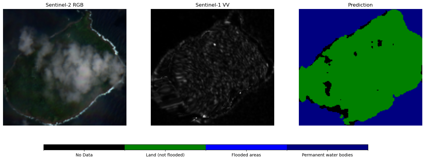
vanuatu_imageryLet’s plot the predictions with the matching VV and RGB images.
region_idx = 15 #10
s1_data, s2_data = vanuatu_imagery[region_idx]

# Normalize VV
vv = s1_data["vv"].values
vv = (vv - vv.min()) / (vv.max() - vv.min())

# Normalize RGB
rgb = np.stack([s2_data["red"], s2_data["green"], s2_data["blue"]], axis=-1) #.values
rgb = (rgb - rgb.min()) / (rgb.max() - rgb.min())  # Normalize to 0–1

# Model prediction
img = torch.as_tensor(s1_data.to_array().values, device='cpu').unsqueeze(0)
output = model(img)
prediction = torch.softmax(output, dim=1).squeeze(0)
prediction = torch.argmax(prediction, dim=0).cpu().numpy()

# Resize prediction to match vv
if prediction.shape != vv.shape:
    prediction = resize(
        prediction, vv.shape, order=0, preserve_range=True, anti_aliasing=False
    ).astype(np.uint8)

# Define discrete colormap
cmap = mcolors.ListedColormap(["black", "green", "blue", "navy"])  # Colors for classes 0-3
bounds = [0, 1, 2, 3, 4]  # Boundaries between color levels
norm = mcolors.BoundaryNorm(bounds, cmap.N)

# Plot
fig, axes = plt.subplots(1, 3, figsize=(18, 6))

# Sentinel-2 RGB
axes[0].imshow(rgb)
axes[0].set_title("Sentinel-2 RGB")

# Sentinel-1 VV
axes[1].imshow(vv, cmap="gray")
axes[1].set_title("Sentinel-1 VV")

# Prediction with colormap
im = axes[2].imshow(prediction, cmap=cmap, norm=norm)
axes[2].set_title("Prediction")

# Adjust layout to make space for the legend
fig.subplots_adjust(bottom=0.2)

# Create a separate axis for the colorbar below the plots
cbar_ax = fig.add_axes([0.2, 0.08, 0.6, 0.03])  # [left, bottom, width, height]
cbar = fig.colorbar(im, cax=cbar_ax, orientation="horizontal")

# Fix the tick positions to be at class centers
tick_positions = [0.5, 1.5, 2.5, 3.5]  # Midpoints of the class ranges
cbar.set_ticks(tick_positions)
cbar.set_ticklabels([class_labels[i] for i in range(4)])

for ax in axes:
    ax.axis("off")

plt.show()
Finally, let’s vectorize our predictions to create polygons and write those to a GeoJSON file.
# Initialize a list to store results
vectorized_predictions = []

for idx, (s1_data, s2_data) in enumerate(vanuatu_imagery):
    polygon = admin_boundaries_gdf.iloc[idx].geometry  # Get the region geometry

    # Normalize Sentinel-1 VV
    vv = s1_data["vv"].values
    vv = (vv - vv.min()) / (vv.max() - vv.min())

    # Model Prediction
    img = torch.as_tensor(s1_data.to_array().values, device="cpu").unsqueeze(0)
    output = model(img)
    prediction = torch.softmax(output, dim=1).squeeze(0)
    prediction = torch.argmax(prediction, dim=0).cpu().numpy()

    # Vectorize Prediction using rasterio
    mask = prediction > 0  # Exclude "No Data" class (class 0)
    shapes_gen = shapes(prediction.astype(np.int16), mask=mask, transform=s1_data.rio.transform())

    # Convert raster shapes into GeoDataFrame features
    for geom, value in shapes_gen:
        class_id = int(value)
        vectorized_predictions.append({
            "geometry": shape(geom),
            "region": admin_boundaries_gdf.iloc[idx]["iname"],
            "class_id": class_id,
            "class_name": class_labels.get(class_id, "Unknown")
        })

# Create a GeoDataFrame
gdf_predictions = gpd.GeoDataFrame(vectorized_predictions)
gdf_predictions.set_crs(epsg=32758, inplace=True) # WGS 84 / UTM zone 58S

# Save as GeoJSON
gdf_predictions.to_file("vanuatu_flood_predictions.geojson", driver="GeoJSON")

print("GeoJSON file saved: vanuatu_flood_predictions.geojson")
GeoJSON file saved: vanuatu_flood_predictions.geojson
You can see why we set the coordinate reference system to EPSG=32758 below. It is that which the Sentinel-1 data is assigned to.
s1_data.rio.crsCRS.from_wkt('PROJCS["WGS 84 / UTM zone 59S",GEOGCS["WGS 84",DATUM["WGS_1984",SPHEROID["WGS 84",6378137,298.257223563]],PRIMEM["Greenwich",0],UNIT["degree",0.0174532925199433,AUTHORITY["EPSG","9122"]],AUTHORITY["EPSG","4326"]],PROJECTION["Transverse_Mercator"],PARAMETER["latitude_of_origin",0],PARAMETER["central_meridian",171],PARAMETER["scale_factor",0.9996],PARAMETER["false_easting",500000],PARAMETER["false_northing",10000000],UNIT["metre",1],AXIS["Easting",EAST],AXIS["Northing",NORTH],AUTHORITY["EPSG","32759"]]')gdf_predictions.head(10)We can plot all of the region-wise predicitons in their vector format below.
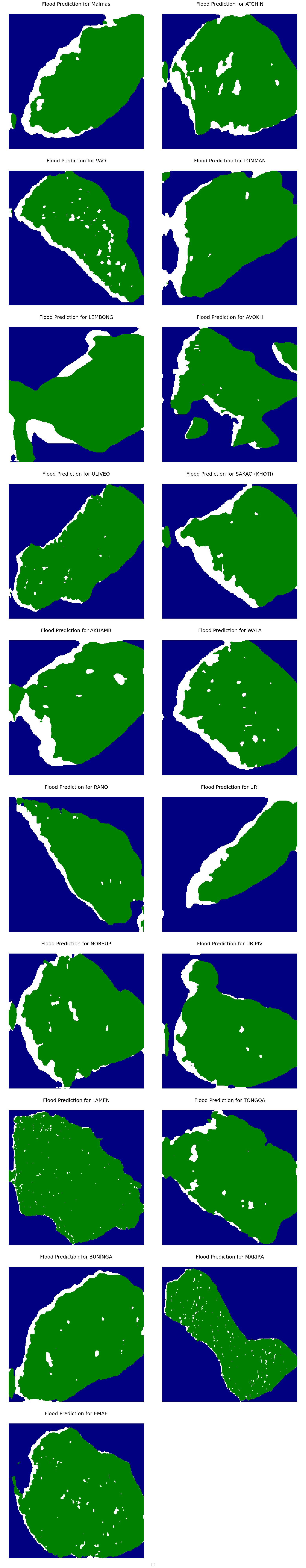
# Define a colormap for class names
class_colors = {
    "No Data": "black",
    "Land (not flooded)": "green",
    "Flooded areas": "blue",
    "Permanent water bodies": "navy"
}

cmap = mcolors.ListedColormap(class_colors.values())
bounds = range(len(class_colors) + 1)
norm = mcolors.BoundaryNorm(bounds, cmap.N)

# Get unique regions
regions = gdf_predictions["region"].unique()
num_regions = len(regions)

# Set up grid layout (2 columns, rows calculated dynamically)
cols = 2
rows = math.ceil(num_regions / cols)  # Round up to fit all regions

# Increase figure size to make each subplot larger
fig, axes = plt.subplots(rows, cols, figsize=(16, rows * 8))  # Adjusted figure size

# Flatten axes array if there's more than 1 row
axes = axes.flatten() if num_regions > 1 else [axes]

for i, region in enumerate(regions):
    ax = axes[i]

    # Filter data for the specific region
    region_predictions = gdf_predictions[gdf_predictions["region"] == region]

    # Plot predictions
    region_predictions.plot(
        column="class_id",
        cmap=cmap,
        norm=norm,
        legend=False,  # Avoid duplicate legends
        ax=ax
    )

    ax.set_title(f"Flood Prediction for {region}", fontsize=18)
    ax.axis("off")

# Remove empty subplots if num_regions < rows * cols
for j in range(i + 1, len(axes)):
    fig.delaxes(axes[j])

# Add a single legend outside the plots
fig.legend(handles=ax.collections, labels=class_colors.keys(), loc="lower center", ncol=4, fontsize=14)

plt.tight_layout()
plt.show()
/tmp/ipykernel_396/1543425869.py:51: UserWarning: Mismatched number of handles and labels: len(handles) = 1 len(labels) = 4
  fig.legend(handles=ax.collections, labels=class_colors.keys(), loc="lower center", ncol=4, fontsize=14)
/tmp/ipykernel_396/1543425869.py:51: UserWarning: Legend does not support handles for PatchCollection instances.
A proxy artist may be used instead.
See: https://matplotlib.org/stable/users/explain/axes/legend_guide.html#controlling-the-legend-entries
  fig.legend(handles=ax.collections, labels=class_colors.keys(), loc="lower center", ncol=4, fontsize=14)