Land Use / Land Cover Segmentation Using Sentinel-2 and Random Forest - ML training for Climate Change and Natural Disasters

This workflow demonstrates how to use Sentinel-2 satellite imagery for segmenting land use / land cover (LULC) using a Random Forest classifier. We focus on detecting planted forests by integrating ground truth forest areas from the National Forest Classification Dataset (LULC) from 2018.

In this notebook, we will demonstrate the following:

Data Acquisition:
- We use Sentinel-2 L2A data (Level-2A provides surface reflectance) accessed via the AWS STAC catalog. The search is filtered by parameters like a region of interest (AOI), time range, and cloud cover percentage to obtain suitable imagery.
Preprocessing:
- The Sentinel-2 imagery contains several spectral bands (e.g., Red, Green, Blue, and Near-Infrared). These are extracted and combined into a single dataset for analysis. Additionally, the imagery is masked to remove areas outside the AOI and focus on the relevant pixels.
Feature Extraction:
- Features for the classifier are extracted from the Sentinel-2 spectral bands. Here, we will use the reflectance values from the Red, Green, Blue, and Near-Infrared (NIR) bands. We will mask out clouds from these bands before further analysis.
Ground Truth Data Integration:
- A shapefile containing polygons attributed by land cover/land use is loaded into a GeoDataFrame. This allows us to create multi-class labels for the pixels in the Sentinel-2 imagery.
Data Splitting:
- To ensure correct model training, we split the features and labels into training (80%) and testing (20%) sets. A ‘seed’ value is used for the random number generator to ensure this random split is reproducible.
Random Forest Classification:
- We train a Random Forest classifier to predict planted forest areas. The n_estimators parameter is a key hyperparameter, determining the number of decision trees in the forest. Random Forest leverages the collective wisdom of multiple decision trees to make accurate predictions.
Prediction:
- We will use the trained classifier to predict the likelihood of lulc types for each pixel in the image.
Evaluation:
- After making predictions on the test set, we evaluate the model’s performance using metrics such as accuracy and F1-score. This allows us to assess the performance of the Random Forest model and the effectiveness of the selected features.
Visualization:
- We visualize the predictions by plotting the classified map, where lulc types are indicated by specific color codes.

At the end, you will have trained a model to predict land use + land cover in Vanuatu.

import geopandas as gpd
import matplotlib.pyplot as plt
import numpy as np
import odc.stac
import xarray as xr
from geocube.api.core import make_geocube
from pystac_client import Client
from sklearn.ensemble import RandomForestClassifier
from sklearn.metrics import accuracy_score, ConfusionMatrixDisplay
from sklearn.model_selection import train_test_split

Data Acquisition¶

Let’s read the LULC data into a GeoDataFrame.

A GeoDataFrame is a type of data structure used to store geographic data in Python, provided by the GeoPandas library. It extends the functionality of a pandas DataFrame to handle spatial data, enabling geospatial analysis and visualization. Like a pandas DataFrame, a GeoDataFrame is a tabular data structure with labeled axes (rows and columns), but it adds special features to work with geometric objects, such as:

a geometry column
a CRS
accessibility to spatial operations (e.g. intersection, union, buffering, and spatial joins)

lulc_gdf = gpd.read_file("./lulc_utm_subset.geojson")

We can check out the attributes associated with this dataset:

lulc_gdf.columns

Let’s see which classes are available to us in the most recent LULC column.

lulc_gdf.lulc_2018.unique()

And view a subset of the data (shuffled for more variety in the 10 samples):

lulc_gdf.sample(frac=1).head(10)

We can also plot the vector dataset, and color code the polygons by the relevant LULC column.

lulc_gdf.plot(column='lulc_2018')

Let’s get the bounds of the dataset to provide in a query for overlapping satellite imagery.

# Get the bounds of the forest polygons to define the AOI
aoi = lulc_gdf.to_crs(epsg="4326").total_bounds  # (minx, miny, maxx, maxy)
aoi

We are going to search the AWS open data STAC API just as before for Sentinel-2 L2A atmospherically corrected satellite imagery.

# Access AWS STAC for Sentinel-2 Data
aws_stac_url = "https://earth-search.aws.element84.com/v1"
stac_client = Client.open(aws_stac_url)

# Search Sentinel-2 data on AWS with cloud cover less than 20%
s2_search = stac_client.search(
    collections=["sentinel-2-l2a"],
    bbox=list(aoi),
    datetime="2018-01-01/2018-12-31", 
    query={"eo:cloud_cover": {"lt": 5}}  # Filter by cloud cover < 5%
)

# Retrieve all items from search results
s2_items = s2_search.item_collection()

len(s2_items)

Preprocessing¶

Now that we have a list of relevant image scenes, let’s read the relevant assets into an xarray.Dataset. We will chunk the data with dask to increase processing speed and efficiency.

s2_data = odc.stac.load(
    items=s2_items,
    bands=["red", "green", "blue", "nir", "scl"],
    bbox=aoi,
    chunks={'x': 1024, 'y': 1024, 'bands': -1, 'time': -1},
    resolution=80,
)

s2_data

Let’s define our no data value.

s2_data_nodata = s2_data["scl"].nodata
s2_data_nodata

Also, width and height (in pixel space, NOT latitude and longitude).

width, height = s2_data.x.size, s2_data.y.size

width, height

We will also need to know the CRS for the satellite imagery.

epsg = s2_data.rio.crs.to_epsg()

Feature Extraction¶

Now we will proceed with feature extraction, which will entail selection for the bands we will use for training an LULC model (the features). Cloud cover can obstruct the signal in these bands, so we will mask those out before creating a temporal composite.

bands = ['red', 'green', 'blue', 'nir']

cloud_classes = [3, 7, 8, 9, 10]  # Cloud-related SCL classes
cloud_mask = s2_data['scl'].isin(cloud_classes)
s2_data_masked = s2_data[bands].where(~cloud_mask, drop=False)  # Keep all pixels

#nodata_mask = s2_data['scl'].isin(s2_data_nodata)
#s2_data_composite = s2_data[bands].where(~s2_data_nodata, drop=False)

# Average across the time dimension
s2_data_composite = s2_data_masked.median(dim='time')

s2_data_composite[["red", "green", "blue"]].to_array("band").plot.imshow(rgb="band", robust=True, size=5, aspect=1)

cloud_mask.median(dim='time').plot()

Ground Truth Data Integration¶

Now that we have our features, let’s obtain our labels. The first step is to generate numerical equivalents for the string classes. We index the valid classes starting from 1 so as to reserve 0 for no data pixels.

# Get unique classes and assign integers
unique_classes = lulc_gdf['lulc_2018'].unique()
class_mapping = {cls: i+1 for i, cls in enumerate(unique_classes)}

# Add numerical column
lulc_gdf['lulc_2018_numeric'] = lulc_gdf['lulc_2018'].map(class_mapping)

print(lulc_gdf.lulc_2018.unique(), lulc_gdf.lulc_2018_numeric.unique())

We need these in raster format. Thus, we will inctroduce a new tool called geocube that “rasterizes” vector data into a gridded xarray.Dataset that matches up with the raster features!

We start by making sure the LULC vector data is projected in the same CRS as the satellite imagery.

lulc_gdf = lulc_gdf.to_crs(epsg=epsg)

# Define the resolution and bounds based on Sentinel-2 features
resolution = s2_data.rio.resolution()
bounds = s2_data.rio.bounds()

# Rasterize the vector dataset to match Sentinel-2
rasterized_labels = make_geocube(
    vector_data=lulc_gdf,
    measurements=["lulc_2018_numeric"], 
    like=s2_data,  # Align with the features dataset
)

# The rasterized output is an xarray.Dataset
print(np.unique(rasterized_labels["lulc_2018_numeric"].values))

Let’s convert no data encoded as nan to zero. We need all pixels to have a numeric value.

rasterized_labels = rasterized_labels.where(~np.isnan(rasterized_labels), other=0)  # Replace NaNs with 0

print(np.unique(rasterized_labels["lulc_2018_numeric"].values))

We also need our labels to be of type integer, not float.

rasterized_labels = rasterized_labels.astype(int)

print(np.unique(rasterized_labels["lulc_2018_numeric"].values))

Let’s plot our new labels xarray.Dataset.

rasterized_labels["lulc_2018_numeric"].plot()

Now we have to flatten the feature and labels datasets because the random forest segmentor expects the inputs to be 1-dimensional.

features = s2_data_composite.to_array().stack(flattened_pixel=("y", "x")).transpose("flattened_pixel", "variable")
labels = rasterized_labels.to_array().stack(flattened_pixel=("y", "x")).transpose("flattened_pixel", "variable").squeeze()

Let’s check the new shapes.

features.shape, labels.shape

Data Splitting¶

Now that we have the arrays flattened, we can split the datasets into training and testing partitions. We will reserve 80 percent of the data for training, and 20 percent for testing.

# Split data into training and testing sets
X_train, X_test, y_train, y_test = train_test_split(features, labels, test_size=0.2, random_state=42)

len(X_train), len(X_test), len(y_train), len(y_test)

Random Forest Classification¶

Now we will set up a small random forest classifider with 10 trees. We use a seed (random_state) to ensure reproducibility. Calling the .fit() method on the classifier will initiate training.

%%time
# Train a Random Forest classifier
clf = RandomForestClassifier(n_estimators=10, random_state=42, n_jobs=-1)
clf.fit(X_train, y_train)

Prediction¶

Once the classifier is finished training, we can use it to make predictions on our test dataset.

# Test the classifier
y_pred = clf.predict(X_test)

Evaluation¶

It’s important to know how well our classifier performs relative to the true labels (y_test). For this, we can calculate the accuracy metric to measure agreement between the true and predicted labels.

# Evaluate the performance (you can use metrics like accuracy, F1-score, etc.)
print("Accuracy:", accuracy_score(y_test, y_pred))

We can also plot a confusion matrix to explore per-class performance.

ConfusionMatrixDisplay.from_predictions(y_true=y_test, y_pred=y_pred)

Notice that we see a high variability in the performance across classes. This is likely due to a class imbalance or inter-class differentiation challenge within our training dataset. It’s possible that augmentations or class revision may help to address this.

Visualization¶

If we want to generate predictions for the entire dataset in order to plot a map of predicted LULC for the entire area of interest, we can do this using the full (un-partitioned) features dataset.

y_pred_full = clf.predict(features)

np.unique(y_pred_full)

Now, we will reshape the predictions back to the 2-dimensional shape and plot the results.

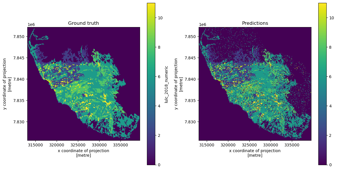
predicted_map = y_pred_full.reshape((height, width))  # Reshape back to original dimensions

# Create an Xarray DataArray
predicted_map_xr = xr.DataArray(data=predicted_map, coords=rasterized_labels.coords)

fig, axes = plt.subplots(1, 2, figsize=(12, 6))

rasterized_labels["lulc_2018_numeric"].plot(ax=axes[0], cmap="viridis")
axes[0].set_title("Ground truth")
axes[0].set_aspect('equal')

predicted_map_xr.plot(ax=axes[1], cmap="viridis")
axes[1].set_title("Predictions")
axes[1].set_aspect('equal')

plt.tight_layout()
plt.show()

We can save the predicted LULC image to a GeoTIFF image.

predicted_map_xr.rio.to_raster(raster_path="predicted_lulc.tif", driver="COG")