Intro to Selecting and Processing Raster Data

This workflow introduces how to search for, acquire and process raster data efficiently. Specfically, we demonstrate finding Sentinel-2 satellite imagery relevant for an area and time defined by a subset of Vanuatu with the same temporal range as the VBoS-provided GIS data (2018).

Note: some portions of this notebook are inspired by the Introduction to Geospatial Raster and Vector Data with Python course.

Main Objectives¶

• Access Sentinel-2 data: Locate and retrieve relevant Sentinel-2 data for a specific area and timeframe via STAC.

• Inspect and visualize raster data: Examine metadata, including projections, bands, dimensions no data pixels. Plot raster data correctly.

• Process multi-spectral raster data: Work with vector data to establish bounds, manage coordinate systems, and set up the area of interest (AOI).

• Interpret time-series raster data: Learn to explore the time dimension for raster data and search for temporal patterns.

• Cloud masking and compositing: Handle clouds and create composites from multiple image scenes.

• Speed up raster processing with Dask: Learn how to optimize raster processing steps using a parallel processing library.

At the end, you’ll be able to efficiently process raster imagery for a region and time of interest!

Accessing raster data¶

First let’s start by defining a geometry for a subset of Vanuatu. We will use this to obtain geographic bounds to select and acquire raster data.

Note that we set the coordinate reference system (CRS) to the projection that is used to load web map tiles and store coordinate metadata in the STAC catalog, EPSG:4326 (WGS 84).

The subset is located in the following region of Vanuatu.

Now let’s actually search for and retrieve some raster data.

STAC, which stands for SpatioTemporal Asset Catalog, is an open standard specification designed to organize and describe geospatial assets in a consistent manner. It has become a crucial development in the geospatial industry as it establishes a standard language and structure for describing geospatial data. Ultimately, we use STAC for indexing earth observation data, along with associated metadata for efficient search and access.

You can explore available datasets archived with this spec via the STAC browser. Generally, this resource provides an up-to-date overview of existing STAC catalogs.

Let’s visit and select the “Earth Search” catalog, which serves as the entry point for accessing the archive of Sentinel-2 images hosted on AWS.

To locate the API URL for a catalog in the STAC browser, click the “Source” button on the top-right corner. This URL grants access to the catalog’s data. For example, in the Earth Search STAC catalog, we can see that the API URL is:

In the following steps, we request scenes from the Sentinel-2 L2A collection, which contains Sentinel-2 data products pre-processed to Level 2A (bottom-of-atmosphere reflectance) and stored in Cloud Optimized GeoTIFF (COG) format.

In the next steps, we will request scenes from the Sentinel-2 L2A collection. These Sentinel-2 data products have been processed to Level 2A, which correlates with bottom-of-atmosphere reflectance. Also worth noting, these image scenes are conveniently stored in a format optimized for cloud storage: Cloud Optimized GeoTIFF (COG).

Cloud Optimized GeoTIFFs (COGs) are a type of GeoTIFF that incorporate features making them particularly effective for cloud storage and online applications. COGs retain the standard GeoTIFF format but are specially structured to enhance remote access. A key aspect of this structure is the organization of data into “blocks,” allowing specific parts of the file to be accessed through HTTP requests, so users don’t have to download the entire file. Additionally, COGs often include “overviews”—multiple lower-resolution versions of the image—enabling users to quickly retrieve less detailed versions if high resolution is unnecessary, which greatly reduces data transfer times.

We specifically search for all available Sentinel-2 scenes in the sentinel-2-l2a collection that meet the following conditions:

• intersect with a given bounding box (based on the boundaries of the area of interest);

• were captured between January 1, 2018, and December 31, 2018;

• have less than 5% cloud cover;

• have less than 25% invalid pixels.

Note: At this stage, we’ve only retrieved metadata, meaning no images have been loaded into memory yet. Keep in mind, though, that even metadata can amount to a lot of memory when there are many images that fit the search criteria! To manage this, it’s possible to set a cap on the number of search results by providing another parameter limit=n where n is the maximum allowed number of items to be returned.

Now that we’ve executed the query to find image scenes meeting our search criteria, we can determine how many that is with the following .matched() method. Keep in mind that this result may vary as more data is continually added to the respective catalog):

Which should equate to the number of items collected:

Each item correlates with one image scene for which the metadata contains attributes such as the scene’s geometry and image capture time, to name a few. These attributes can be accessed through the item’s properties.

We can see an example for the first item in the search results:

As previously mentioned, we have only retrieved metadata. Now, we will access the actual rasters (image pixels) for the scenes. In STAC terminology, the image data itself is referred to as “assets”, and for any given image, there is one asset per band. One simple method for reading the image data is through the URLs accessible in the item’s assets attribute.

We can see a description of the available assets for the respective sensor/instrument like so:

The Sentinel-2 L2A data product includes several assets: raster files representing each optical band captured by the multispectral instrument, a thumbnail true-color image (“visual”) image, as well as metadata from the instrument and scene classification data (“SCL”). Let’s gather the URLs for these assets.

That URL represents the location of the image in cloud storage. As it is remote raster data, we will use a library that allows us to directly access it without having to download the image to our file system first. This library is called rioxarray.

Optionally, we can then save the raster data to a file on disk if needed:

Since processing large rasters can be time-consuming (for example, the 10-meter NIR band has over 100 million pixels), it’s often more efficient to work with a smaller subset of the data. Fortunately, because the raster is in Cloud Optimized GeoTIFF (COG) format, we can download just the portion we need! Let’s first check the internal tile size for this band of the COG:

In this case, we specify that we want to download the first band in the TIFF file and extract a subset by slicing the width and height dimensions.

We can read the newly saved image subset and confirm the size is what we expect:

Reading raster data¶

In this section, we cover the core principles, tools, and metadata/raster attributes necessary for handling raster data in Python. We will also explore common ways of managing missing or invalid data values.

The rioxarray library will be our primary tool for working with raster data in this lesson. It builds upon the functionality of rasterio (a package for working with raster data) and xarray (for multi-dimensional arrays). rioxarray, simply put, extends xarray by adding higher-level functions, such as open_rasterio for reading raster datasets, and provides additional methods to xarray objects like Dataset and DataArray that specifically enable geospatial operations. These methods, available through the rio accessor, become accessible in xarray once rioxarray is imported.

For demonstration, we’ll focus on the first scene retrieved and load the nir09 band. This can be done by using the rioxarray.open_rasterio() function with the band asset’s Hypertext Reference (href, or URL).

We can quickly inspect the shape and attributes of the newly opened nir09 dataset we titled raster_vanu_b9 by printing the variable name.

The initial call to rioxarray.open_rasterio() retrieves the file from either local or remote storage, returning a xarray.DataArray. As noted, this object is assigned to a variable like raster_vanu_b9. While using xarray also returns a xarray.DataArray, it won’t include the geospatial metadata (such as scene geometry and projection). You can apply NumPy functions or Python’s math operators to a xarray.DataArray just as you would with a NumPy array, but without rioxarray you can’t make use of any geospatial information.

The output shows the variable name of the xarray.DataArray, and indicates that the data includes 1 band, 1830 rows, and 1830 columns. It also shows the total pixel count and the pixel data type, which is an unsigned integer (uint16).

In addition, thanks to rioxarray, we can see that the DataArray has spatial coordinates (x and y) and band information, with each having its own data type—float64 for spatial coordinates and int64 for bands. Furthermore, rioxarray enables us to see other important geospatial attributes via methods like .rio.crs and .rio.bounds(). Note: most metadata can be accessed directly as attributes (e.g., .rio.crs), but some methods like .rio.bounds() require parentheses to retrieve the information.

The Coordinate Reference System for raster_vanu_b9.rio.crs is returned to be EPSG:32759. The no-data value is set to 0, and the bounding box corners of our raster are returned by the output of .bounds(). The height and width in number of pixels are returned from .rio.height and .rio.width, respectively.

Visualizing raster data¶

We’ve reviewed the attributes of our raster. Now let’s see the raw values of the array with .values:

Printing this provides a quick glimpse of the values in our array (by way of showing pixels just on image corners). Since our raster is loaded in Python as a DataArray type, we can also plot it in a single line, similar to how we would with a pandas DataFrame, using DataArray.plot().

Observe that rioxarray conveniently enables us to plot this raster with spatial coordinates on the x and y axes.

The plot displays the satellite image pixels for the spectral band nir09 over our area of interest. According to the Sentinel-2 documentation, this band has a central wavelength of 945 nm, making it sensitive to water vapor. This band is one of the lower spatial resolution wavelengths captured by the instrument at a spatial resolution of 60 m. This makes it convenient here for quick demonstrations.

It’s important to note that the band=1 in the image title refers to the order of the bands in the DataArray, not the Sentinel-2 band asset nir09.

From a quick glance at the image, we can see that cloudy pixels exhibit high reflectance values, whereas the contrast of other areas is relatively low. This behavior is expected due to the band’s sensitivity to water vapor. However, we can improve color contrast by including the option robust=True, which displays values between the 2nd and 98th percentiles.

This feature generally allows us to adjust the color limits to better accommodate most of the values in the image.

However, it isn’t always sufficient for getting a good representation of the data. In situations where the robust=True option doesn’t work, you can also manually set the vmin and vmax parameters to customize the value range. For instance, you can plot values between 100 and 7000:

Now, if we want to plot a subset of this image more focused on the land masses, we can select a regin of pixels again. Let’s look at the internal tiling for this band of the COG:

Notice that the tile size is smaller because the resolution for this band (nir09) is lower (60 meters) than that of the nir (10 meters).

Deciphering the Raster Coordinate Reference System (CRS)¶

Another important piece of information we want to examine is the Coordinate Reference System (CRS), which can be accessed using .rio.crs. We will explore how the characteristics of the CRS are represented in our data file and their significance. To view the CRS string associated with our DataArray, we can utilize the rio accessor to obtain the crs attribute.

EPSG codes offer a concise way to represent specific coordinate reference systems (CRS). However, for more comprehensive details about a CRS, such as its units of measurement, the pyproj library can be used. This library is specifically designed to handle the definition and function of coordinate reference systems.

The CRS class from the pyproj library enables us to create a CRS object. We can retrieve specific information about a CRS from this, as well as obtain a basic summarization of the associated CRS.

One especially valuable attribute is area_of_use, which indicates the geographic boundaries for which the CRS is designed to be applied.

The pyproj CRS summary encompasses all the individual elements of the CRS that Python or other GIS software may require.

For our example, the projection name is UTM zone 59S (the UTM system comprises 60 zones, each spanning 6 degrees of longitude) with an underlying datum of WGS84. The CRS utilizes a Cartesian coordinate system with two axes, easting and northing, measured in meters. This projection is applicable for a specific range of longitudes, from 168°E to 174°E, in the southern hemisphere (from 80.0°S to 0.0°S). The coordinate operation describes how the coordinates are projected (if applicable) onto a Cartesian (x, y) plane. The Transverse Mercator projection is effective for regions with narrow longitudinal widths, as is the case with UTM zones. The datum serves as the reference point for coordinates. WGS 84 is a widely used datum. It’s important to note that the zone is specific to the UTM projection, and not all CRSs will have a designated zone.

Calculate Raster Statistics¶

Knowing basic statistical values of a raster dataset can be valuable. We can obtain some, such as minimum, maximum, mean, and standard deviation quite easily for xarray.DataArrays like so:

So with that, we can get key statistical values such as the minimum, maximum, mean, and standard deviation, along with the data type of the pixels. However, if you’re interested in calculating specific quantiles, xarray provides the .quantile() method. For example, to determine the 25th and 75th percentiles, you can try the following:

Dealing with Missing Data¶

Up until now, we’ve visualized a band from a Sentinel-2 scene and computed its statistics. However, it’s essential to factor in missing data. Raster datasets typically include a “no data value” or “nodata.” This value is used for pixels where data is absent, which may occur due to various reasons, such as sensor limitations or gaps in data collection. Often, missing data appears at the raster edges, especially when the data does not cover the entire area being analyzed.

By design, raster datasets have a rectangular shape. Therefore, if the data doesn’t fully cover a region, the pixels at the boundary might be marked as nodata. For instance, sensor data might only cover a portion of a given area, leaving edges with no data.

In this case, the nodata value for the dataset (raster_vanu_b9.rio.nodata) is 0. When we visualized the data or calculated statistics, these missing values were treated the same as valid data. This could result in misleading conclusions—such as a falsely low 25th percentile—because the nodata pixels, which are represented by zeros, can distort the calculation.

To address this and more clearly distinguish missing data, we can use nan to represent these values. This can be done by setting masked=True when loading the raster.

You can also utilize the where function to filter out all the pixels that differ from the raster’s nodata value:

Both methods will convert the nodata value from 0 to nan and thus allow us to recalculate the statistics with the missing data excluded. Additionally, you can use the .values attribute with the statistical functions to obtain only the calculated values, without any of the object metadata.

It’s worth mentioning that replacing 0 with nan to represent missing data will cause a change in the data type of the DataArray from integers to floats. This is an important consideration if the data type plays a crucial role in your specific use case or application.

Incorporating multiple bands¶

Up to this point, we have examined a single-band raster, specifically the nir and subsequently nir09 bands of a Sentinel-2 scene. However, if we want to see an easy-to-interpret RGB “true-color” version of the scene, we can look at the overview (TCI) asset. The Sentinel-2 True Color Image (TCI) is a full-resolution visual representation of the scene. This image is created by combining three specific optical bands—Red, Green, and Blue (RGB)—captured by the Sentinel-2 satellite’s MultiSpectral Instrument (MSI). With a spatial resolution of 10 meters, the TCI provides a detailed, visually intuitive view of the scene’s captured area, assisting with quick assessments and visual analysis. Like the nir09 band, we can load it using:

Note that we provided an argument overview_level=3. For Sentinel-2 COGs, the spatial resolution at different overview levels depends on how much the image is downsampled. Sentinel-2 data products have a native spatial resolution of 10 meters for True Color Image (TCI) bands, but each overview level decreases this resolution by a factor of 2.

If you read the TCI at overview level 3, the spatial resolution is effectively:

• Level -1 (native): 10 meters

• Level 0: 20 meters

• Level 1: 40 meters

• Level 2: 80 meters

• Level 3: 160 meters

When reading GeoTIFFs using the open_rasterio() function and printing the shape, the band number appears first. In the xarray.DataArray object, we can observe that the shape is now (band: 3, y: 687, x: 687). From this, we can easily see the number of bands in the named band dimension. It’s always advisable to check the shape of the raster array you are working with to make sure it meets your expectations, both after reading the image into an array and intermittently as you undergo manipulations of the dataset (e.g. calculating band ratios or warping). Many functions, particularly those used for plotting images, require the raster array to have a specific shape (e.g. 1 or 3 channels ordered a certain way). A very simple way to verify the shape is using the .shape attribute:

You can visualize the multi-band data using the DataArray.plot.imshow() function:

Keep in mind that the DataArray.plot.imshow() function assumes the input DataArray has three channels, which corresponds to the RGB colormap. It is not compatible with image arrays that contain more than three channels. However, you can create a false-color image by substituting RGB channels with others.

As illustrated in the figure above, the true-color image appears stretched. To visualize it with the correct aspect ratio, we can adjust the settings for DataArray.plot.imshow().

Given that the height-to-width ratio is 1:1 (as confirmed by the rio.height and rio.width attributes), let’s set the aspect ratio to 1. For instance, this would be a good example to set the size of the plot to 5 inches and specify aspect=1. Note that when using the aspect argument, you must also provide a size, as stated in the DataArray.plot.imshow() documentation.

Now let’s say we want to work with not just the visual bands, but also some of the others, such as the nir band. We’ll introduce a new tool and method for loading raster data from STAC into an xarray.Dataset called Open Data Cube (ODC) which we imported as odc.

odc features an extension for working with raster data from STAC-compliant catalogues. We will use this to more robustly work with the Sentinel-2 data that we queried for earlier.

In the following cell, we do the following:

1. s2_data = odc.stac.load(...):

   • This line uses the odc library to load data from the Sentinel-2 items we collected metadata for. The load function retrieves the actual raster data.

2. items=s2_items:

   • The s2_items refers to the Sentinel-2 items (scenes) we retrieved earlier from the STAC catalog search. These items contain the metadata and location of the relevant Sentinel-2 data, which will be loaded in this step.

3. bands=["red", "green", "blue", "nir", "scl"]:

   • This specifies the spectral bands to load: Red, Green, Blue, and Near-Infrared (NIR). These are common bands used for analyzing land cover, vegetation health, and generating RGB images. We also include a band that isn’t a necessary a wavelength range, but rather a classification layer (SCL) which we will use to know where cloudy pixels are.

4. bbox=box_coords:

   • The bbox argument defines the Area of Interest (AOI), which is the geographic bounding box of the region we want to load data for (same one as used earlier for the subset of Vanuatu). The AOI is given as a list of coordinates that define the region’s extent: [min_longitude, min_latitude, max_longitude, max_latitude].

5. progress=tqdm:

   • The progress argument links the loading process to tqdm, which provides a progress bar. This is useful when loading large datasets, as it shows how much data has been loaded and gives an indication of how long the process might take.

IMPORTANT: When provided a bbox argument, odc will automatically clip the generated raster to the bounds of the provided extent. This means we only return the pixels that we are actually interested in!

The result, s2_data, is a xarray.Dataset that we can use for further analysis, such as visualization or classification.

The odc.stac.load() function returns an xarray.Dataset instead of an xarray.DataArray because we are loading more than one spectral band (["red", "green", "blue", "nir", "scl"]). A xarray.Dataset is designed to hold a single variable (or band) of data. Since we are loading multiple bands, the function returns a xarray.Dataset, which is essentially a collection of DataArrays, where each DataArray corresponds to one of the requested bands. A xarray.Dataset can be thought of as a container for multiple DataArrays. It can hold multiple variables (e.g., bands like red, green, blue, nir), each with the same or different dimensions and coordinates. In this case, each band (e.g., red, green, etc.) is a separate DataArray within the Dataset.

The xarray.Dataset structure allows you to work with multiple related variables (e.g., bands) in the same space, with shared coordinates (such as latitude, longitude, and time). This makes it easier to perform operations that involve multiple bands, such as stacking them together to create a RGB image or performing multi-band analysis.

If you were loading only a single band, the odc.stac.load() function could return a DataArray, which is more suited to holding a single variable with associated dimensions and coordinates. However, because we requested multiple bands, a xarray.Dataset is the appropriate return type.

Notice that the time dimension is automatically interpreted and correctly lines up with the 7 items we returned from s2_search.matched() and len(s2_items) earlier. This means we have 7 items overlapping the AOI from different image captures with different timestamps. odc doesn’t assume we want to do any manipulation by default on the time dimension so it returns the dataset with the items stacked in a time series.

In order to plot this image, let’s composite the image over time, to produce a temporal depth of 1 where pixels represent the median value over all of the timestamps.

Notice the new shape of the dataset:

Also notice here that the aspect ratio is not perfectly 1:1, but close enough (1.003:1) for use with a 1:1 aspect ratio when plotting. We can plot a true color image from the dataset by specifying the necessary bands.

We can also plot any single band from the dataset like so:

Let’s say we want to take a look at the time series for a single band. We can do this by taking the median value over the spatial dimensions (x and y) for each timestamp and plotting the values.

Then we can extract the time series for one of bands. Near infrared is interesting because it is useful in determing seasonal phenology.

We can plot a line plot for the near infrared median values for each timestamp.

Dealing with cloudy pixels¶

To mask out clouds from Sentinel-2 data, we can use the ‘SCL’ (Scene Classification Layer) band, which includes cloud information. The SCL band classifies each pixel in the Sentinel-2 image, including cloud-related classes such as cloud shadows, medium-probability clouds, high-probability clouds, and cirrus clouds. By masking out these classes, we can remove cloud-covered pixels from the dataset.

First we need to declare the cloud-related SCL classes. The common classes for clouds are:

Cloud Shadows: 3

Low probability clouds: 7

Medium probability clouds: 8

High probability clouds: 9

Thin cirrus: 10

In order to mask out these cloud classes, we’ll create a boolean mask using xarray’s .isin() method.

Now, we will use the cloud mask to filter out cloud-covered pixels in the red, green, blue, and NIR bands.

Let’s plot the cloud-free data to verify the results. To do this, let’s composite the imagery again to get a temporal median.

Now we can plot an image.

The image plot is looking a bit over-exposed. Let’s adjust the value ranges to better fit the raster data.

That looks pretty good! Now we have a cloud-masked composite. We can use this to get a clearer signal of near infrared over time.

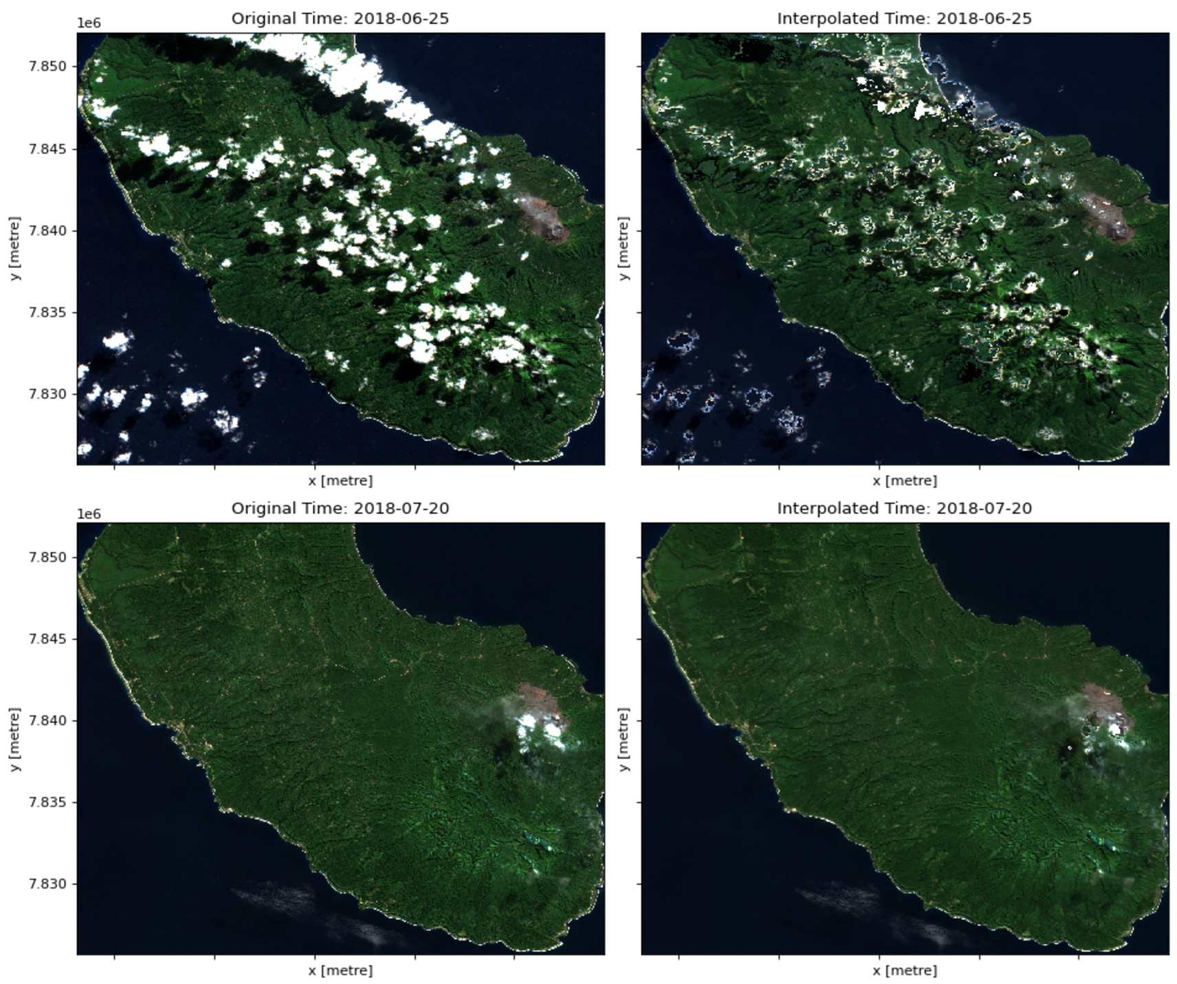
What if we want to interpolate where the cloudy pixels are for each timestamp, however, instead of reducing to a single temporal composite? We can do this using the cloud mask and an interpolation (e.g. linear, nearest neighbor, spline) method on either the spatial (x and y) dimension or time. Combinations of these will imply different overhead and thus varying run times.

For this example, we will interpolate on the time dimension. For the following, we need to get the cloud mask, this time actually changing the values for cloudy pixels to NaN:

We will then introduce a new library, dask, which is used to parallelize expensive operations by chunking data into smaller parts and distributing those across available workers. Here, we select a chunk size based on the shape of the DataArray. The chunk size is a factor that is specific to the size of your data and should closely match any internal tiling paramaters if relevant (as is the case for COGs).

We will also apply downsampling to further reduce the computation time. In practice, you might not want to downsample your data if spatial resolution is very important, but here we do so for the purposes of a quick example. Note that in the downsampling step coarsen() we provide x=4, y=4 which specifies the size of the neighborhood over which to apply an averaging function. In this case, it will take the median value every 4 pixels along the x-axis and every 4 pixels along the y-axis. We also include boundary='trim' which determines how the edges of the DataArray are handled. With boundary='trim', any excess pixels that do not fit into the averaging windows are removed from the result. For example, if the dimensions of cloudy_pixels are not exact multiples of 4, the excess pixels at the edges will be discarded. Lastly, .median() is the coarsening operation. Calling .median() computes the median value of each coarse block defined by the coarsen() method. This results in a new DataArray with a lower spatial resolution, where each pixel represents the median value of a 4x4 block of pixels from the original cloudy_pixels.

On the interpolation algorithm, we use one of the faster options, nearest neighbors. It’s less accurate than alternatives like linear because it samples from a small number of adjacent pixels, but that’s what also makes it relatively faster.

Let’s start with benchmarking time to run without chunking using dask.

Now, let’s chunk the data along the spatial dimensions. We don’t want to chunk on the time dimension, so we tell dask to leave that dimension alone. Dask treats -1 as a special flag that means “do not chunk” or “use the full length of this dimension as a single chunk.” Essentially, -1 is a shorthand to tell Dask that you want to keep the entire dimension in one piece.

Much faster! Let’s plot a result for one of the timestamps.

We can see that the interpolation isn’t exactly good, but this example demonstrates how we can examine time series data and consider challenges like cloud cover whilst improving efficiency with tools like dask!