In this lesson, we will use multi-spectral imagery, cloud-masked and temporally composited, to calculate a comprehensive set of remote sensing indices for characterizing soil health. We’ll summarize the correlations and variance within these indices using Prinicipal Components Analysis (PCA) and calculate a proxy soil health score for each pixel in our composite.
import os
import glob
import math
import pyproj
from datetime import datetime, timedelta
import pandas as pd
import numpy as np
import geopandas as gpd
import rasterio
from rasterio.features import geometry_mask
from sklearn.decomposition import PCA
import tqdm
import xarray as xr
import rioxarray as rxr
import planetary_computer
import pystac_client
from pystac_client import Client
import odc.stac
import matplotlib.pyplot as plt
import matplotlib.colors as mcolors
from shapely.geometry import mapping, shape, MultiPolygon, Point, Polygon, box
from shapely.ops import transform
import dask
import dask.array as da
import dask.delayed
admin_boundaries_gdf = gpd.read_file("./2016_phc_vut_pid_4326.geojson")
#admin_boundaries_gdf = admin_boundaries_gdf.set_index(keys="pname") # set province name as the indexadmin_boundaries_gdfPROVINCE = "SHEFA"
DATERANGE_START = "2025-04-01"
DATERANGE_END = "2025-08-01"admin_boundaries_gdf.columnsIndex(['pid', 'pname', 'geometry'], dtype='object')# Filter to one province (e.g., SHEFA)
#admin_boundaries_gdf = admin_boundaries_gdf.to_crs("EPSG:32759")
province_match = admin_boundaries_gdf[admin_boundaries_gdf["pname"] == PROVINCE]province_matchprovince_match.geometry4 MULTIPOLYGON (((168.30762 -17.77548, 168.30773...
Name: geometry, dtype: geometrymp = province_match.loc[4, "geometry"]
if isinstance(mp, MultiPolygon):
# Sort polygons by area
polys_sorted = sorted(mp.geoms, key=lambda p: p.area)
if len(polys_sorted) >= 3:
#selected = polys_sorted[len(polys_sorted) // 2]
selected = polys_sorted[-5]
elif len(polys_sorted) == 2:
# For just two, pick the larger or smaller depending on definition
selected = polys_sorted[0] # or polys_sorted[1]
else:
selected = polys_sorted[0] # Only one polygon
else:
selected = mp # Already a single polygon
print(len(polys_sorted))
selected33
# Access AWS STAC for Sentinel-2 Data
aws_stac_url = "https://earth-search.aws.element84.com/v1"
stac_client = Client.open(aws_stac_url)
# Search Sentinel-2 data on AWS with cloud cover less than 50%
s2_search = stac_client.search(
collections=["sentinel-2-l2a"],
bbox=selected.bounds,
datetime=f"{DATERANGE_START}/{DATERANGE_END}",
query={"eo:cloud_cover": {"lt": 50}} # Filter by cloud cover < 50%
)# Retrieve all items from search results
s2_items = s2_search.item_collection()len(s2_items)48s2_data = odc.stac.load(
items=s2_items,
bands=["red", "green", "blue", "nir", "swir16", "scl"],
bbox=selected.bounds,
crs="EPSG:32759", #"EPSG:32759",
chunks={'x': 1024, 'y': 1024, 'bands': -1, 'time': -1},
resolution=30
)bands = ['red', 'green', 'blue', 'nir', 'swir16']cloud_classes = [3, 8, 9, 10] # Cloud-related SCL classes
cloud_mask = s2_data['scl'].isin(cloud_classes)
s2_data_masked = s2_data[bands].where(~cloud_mask, drop=False) # Keep all pixels# Average across the time dimension
s2_data_composite = s2_data_masked.median(dim='time')s2_data_composites2_data_composite[["red", "green", "blue"]].to_array("band").plot.imshow(rgb="band", robust=True, size=5, aspect=1)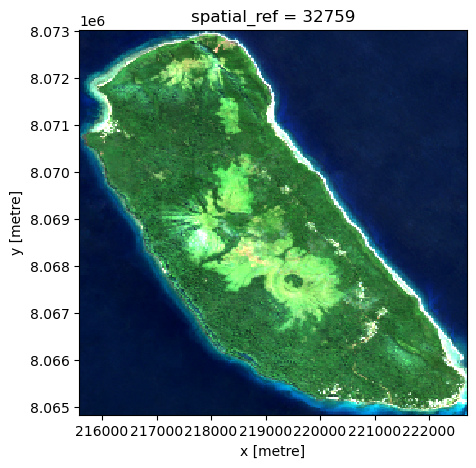
Mask land
project = pyproj.Transformer.from_crs("EPSG:4326", "EPSG:32759", always_xy=True).transform
selected_proj = transform(project, selected)
mask_land = geometry_mask(
geometries=[mapping(selected_proj)],
transform=s2_data_composite.odc.transform,
out_shape=(s2_data_composite.sizes["y"], s2_data_composite.sizes["x"]),
invert=True # We want True = inside the buffer
)mask_land_xr = xr.DataArray(
mask_land,
dims=("y", "x"),
coords={"y": s2_data_composite.y, "x": s2_data_composite.x}
)s2_data_composite_masked = s2_data_composite.where(mask_land_xr)s2_data_composite_masked[["red", "green", "blue"]].to_array("band").plot.imshow(rgb="band", robust=True, size=5, aspect=1)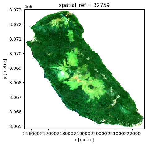
Remote sensing indices for soil health
Monitoring soil health and vegetation condition using satellite imagery relies on various spectral indices that capture moisture, vegetation vigor, soil exposure, and disturbance.
The Normalized Difference Moisture Index (NDMI) assesses vegetation and soil moisture by comparing near-infrared (NIR) and short-wave infrared (SWIR) reflectance, providing insight into water availability crucial for plant growth.
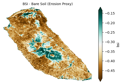
The Bare Soil Index (BSI) highlights areas of exposed or sparsely vegetated soil, which can be indicators of erosion or land degradation.
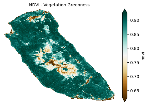
Vegetation vigor and cover are captured by the Normalized Difference Vegetation Index (NDVI), a widely used metric that serves as a proxy for biomass and root activity, thereby indirectly indicating soil protection from erosion.
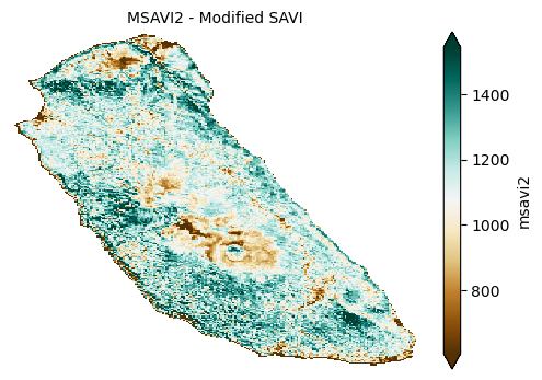
To improve vegetation detection in areas with significant soil exposure, Soil-Adjusted Vegetation Index (SAVI) and its modification MSAVI2 are used; they adjust for soil brightness effects, enabling more accurate vegetation assessment in sparse or mixed soil-vegetation landscapes.
Lastly, the Normalized Burn Ratio (NBR) is sensitive to vegetation disturbance such as fire damage and also reflects exposed soil and land degradation processes. Together, these indices provide a comprehensive view of soil moisture status, vegetation health, bare soil extent, and disturbance—critical factors for assessing soil condition, erosion risk, and ecosystem health in agricultural and natural landscapes.
def compute_ndmi(nir, swir):
    """
    Compute the Normalized Difference Moisture Index (NDMI).

    NDMI measures vegetation and soil moisture by comparing near-infrared (NIR) and short-wave infrared (SWIR) reflectance.

    Formula:
        NDMI = (NIR - SWIR) / (NIR + SWIR)

    Parameters
    ----------
    nir : xarray.DataArray
        Near-infrared reflectance band.
    swir : xarray.DataArray
        Short-wave infrared reflectance band.

    Returns
    -------
    xarray.DataArray
        NDMI values for each pixel.
    """
    return (nir - swir) / (nir + swir)


def compute_bsi(blue, red, nir, swir):
    """
    Compute the Bare Soil Index (BSI).

    BSI identifies bare or sparsely vegetated soil areas, which can indicate erosion or degraded land.

    Formula:
        BSI = ((SWIR + Red) - (NIR + Blue)) / ((SWIR + Red) + (NIR + Blue))

    Parameters
    ----------
    blue : xarray.DataArray
        Blue band reflectance.
    red : xarray.DataArray
        Red band reflectance.
    nir : xarray.DataArray
        Near-infrared reflectance band.
    swir : xarray.DataArray
        Short-wave infrared reflectance band.

    Returns
    -------
    xarray.DataArray
        BSI values for each pixel.
    """
    return ((swir + red) - (nir + blue)) / ((swir + red) + (nir + blue))


def ndvi(red, nir):
    """
    Compute the Normalized Difference Vegetation Index (NDVI).

    NDVI measures vegetation greenness and health.
    NDVI gives vegetation cover health (proxy for root activity, biomass and reduced erosion).

    Formula:
        NDVI = (NIR - Red) / (NIR + Red)

    Parameters
    ----------
    red : xarray.DataArray
        Red band reflectance.
    nir : xarray.DataArray
        Near-infrared reflectance band.

    Returns
    -------
    xarray.DataArray
        NDVI values for each pixel.
    """
    return (nir - red) / (nir + red)


def savi(red, nir, L=0.5):
    """
    Compute the Soil-Adjusted Vegetation Index (SAVI).

    SAVI adjusts NDVI to minimize soil brightness effects, useful in sparse vegetation areas.

    Formula:
        SAVI = ((NIR - Red) * (1 + L)) / (NIR + Red + L)

    Parameters
    ----------
    red : xarray.DataArray
        Red band reflectance.
    nir : xarray.DataArray
        Near-infrared reflectance band.
    L : float, optional
        Soil adjustment factor (default 0.5 for intermediate vegetation cover).

    Returns
    -------
    xarray.DataArray
        SAVI values for each pixel.
    """
    return ((nir - red) * (1 + L)) / (nir + red + L)


def msavi2(red, nir):
    """
    Compute the Modified Soil-Adjusted Vegetation Index 2 (MSAVI2).

    MSAVI2 improves vegetation detection in areas with significant bare soil by removing the need for a soil adjustment factor.

    Formula:
        MSAVI2 = [2 * NIR + 1 - sqrt((2 * NIR + 1)^2 - 8 * (NIR - Red))] / 2

    Parameters
    ----------
    red : xarray.DataArray
        Red band reflectance.
    nir : xarray.DataArray
        Near-infrared reflectance band.

    Returns
    -------
    xarray.DataArray
        MSAVI2 values for each pixel.
    """
    a = 2 * nir + 1
    b = 2 * (nir**2 - nir * red)
    return (a - np.sqrt(a**2 - b)) / 2


def nbr(nir, swir16):
    """
    Compute the Normalized Burn Ratio (NBR).

    NBR detects burned areas and vegetation disturbance.
    Can also indicate exposed soil and land degradation.

    Formula:
        NBR = (NIR - SWIR) / (NIR + SWIR)

    Parameters
    ----------
    nir : xarray.DataArray
        Near-infrared reflectance band.
    swir16 : xarray.DataArray
        Short-wave infrared reflectance band (SWIR1).

    Returns
    -------
    xarray.DataArray
        NBR values for each pixel.
    """
    return (nir - swir16) / (nir + swir16)


s2_data_composite_masked = s2_data_composite_masked.assign(
    ndmi=compute_ndmi(s2_data_composite_masked['nir'], s2_data_composite_masked['swir16']),
    bsi=compute_bsi(
        s2_data_composite_masked['blue'],
        s2_data_composite_masked['red'],
        s2_data_composite_masked['nir'],
        s2_data_composite_masked['swir16']
    ),
    ndvi=ndvi(s2_data_composite_masked['red'], s2_data_composite_masked['nir']),
    savi=savi(s2_data_composite_masked['red'], s2_data_composite_masked['nir']),
    msavi2=msavi2(s2_data_composite_masked['red'], s2_data_composite_masked['nir']),
    nbr=nbr(s2_data_composite_masked['nir'], s2_data_composite_masked['swir16'])
)


def plot_index(index_data, title, cmap='BrBG'):
    plt.figure(figsize=(6, 4))
    index_data.plot(cmap=cmap, robust=True)  # robust=True avoids outlier influence
    plt.title(title, fontsize=10)
    plt.axis('off')
    plt.show()


plot_index(s2_data_composite_masked['ndmi'], 'NDMI - Soil Moisture Indicator')
plot_index(s2_data_composite_masked['bsi'], 'BSI - Bare Soil (Erosion Proxy)')
plot_index(s2_data_composite_masked['ndvi'], 'NDVI - Vegetation Greenness')
plot_index(s2_data_composite_masked['savi'], 'SAVI - Soil-Adjusted Vegetation Index')
plot_index(s2_data_composite_masked['msavi2'], 'MSAVI2 - Modified SAVI')
plot_index(s2_data_composite_masked['nbr'], 'NBR - Disturbance/Burn Ratio')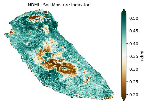


PCA analysis
Let’s search for the dominant pattern of variation across our indices.
Our PCA’s first principal component (PC1) will represent the dominant combined variation in soil moisture, vegetation greenness, soil adjustment, and disturbance indices.
PC1 is a linear combination of all your input bands/indices weighted to explain the maximum variance in the data. Since we included vegetation and soil indices, PC1 often reflects a gradient between soil and vegetation characteristics. For example, it might differentiate areas with healthy, dense vegetation (high NDVI, high moisture) from areas dominated by bare or sparse soil (high BSI, low NDVI). Pixels with high PC1 scores might correspond to lush, healthy vegetation or moist soils; pixels with low PC1 scores might correspond to bare soil, dry or degraded areas.
Goal: to reduce multiple correlated bands and indices into a single composite index capturing the main “soil-vegetation health axis.” This should help summarize complex spectral information into one interpretable value per pixel.
stack = np.stack([s2_data_composite_masked[v].values for v in
['ndmi','bsi','ndvi','msavi2','nbr']]) # shape (bands, t, y, x)stack.shape(5, 273, 237)What the PC1 likely represents with these indices:
PC1 combines moisture, vegetation health, and disturbance info into one axis that captures the biggest variation in your scene.
Areas with high PC1 scores likely correspond to healthy, moist, undisturbed vegetation. Areas with low PC1 scores likely correspond to bare soil, dry areas, or disturbed/affected vegetation.
| Index | Meaning | Expected contribution to PC1 |
|---|---|---|
| NDMI (Normalized Difference Moisture Index) | Soil/vegetation moisture | Higher values → more moisture → likely positive loading |
| BSI (Bare Soil Index) | Bare soil presence | Higher values → more bare soil → usually negative loading (since bare soil = poorer vegetation/health) |
| NDVI (Normalized Difference Vegetation Index) | Vegetation greenness | Higher values → greener vegetation → positive loading |
| SAVI (Soil Adjusted Vegetation Index) | Vegetation with soil adjustment | Similar to NDVI but corrects soil influence → positive loading |
| MSAVI2 (Modified Soil Adjusted Vegetation Index 2) | Vegetation with optimized soil adjustment | Also vegetation indicator → positive loading |
| NBR (Normalized Burn Ratio) | Vegetation disturbance (e.g., fire) | Lower values indicate disturbance; higher values healthy → positive loading expected |
D, Y, X = stack.shape

# flatten spatial dims to samples: (N, D) where N = Y*X
stack_reshaped = stack.reshape(D, Y * X).T  # shape (N, D)

# Create mask for rows without any NaNs
valid_mask = ~np.isnan(stack_reshaped).any(axis=1)

# Filter valid rows only
stack_valid = stack_reshaped[valid_mask]

# Optional: sample if too large
max_samples = 10000
if stack_valid.shape[0] > max_samples:
    idx = np.random.choice(stack_valid.shape[0], max_samples, replace=False)
    pca_data = stack_valid[idx]
else:
    pca_data = stack_valid

# Run PCA on valid data only
pca = PCA(n_components=2)
pca.fit(pca_data)

# Transform all valid pixels
pca_scores_valid = pca.transform(stack_valid)

# Prepare full array with NaNs for invalid pixels
pca_scores = np.full((Y * X, 2), np.nan)
pca_scores[valid_mask] = pca_scores_valid

# reshape PC1 back to (Y, X)
pc1 = pca_scores[:, 0].reshape(Y, X)

# create DataArray for PC1
pc1_da = xr.DataArray(
    pc1,
    coords={
        'y': s2_data_composite_masked['y'],
        'x': s2_data_composite_masked['x']
    },
    dims=['y', 'x'],
    name='soil_vegetation_axis_PC1'
)

# reshape PC1 back to (Y, X)
pc2 = pca_scores[:, 1].reshape(Y, X)

# create DataArray for PC1
pc2_da = xr.DataArray(
    pc2,
    coords={
        'y': s2_data_composite_masked['y'],
        'x': s2_data_composite_masked['x']
    },
    dims=['y', 'x'],
    name='soil_vegetation_axis_PC1'
)

# plot
ax = pc1_da.plot(cmap='RdYlGn', robust=True, figsize=(10, 6))
#ax.set_title('Soil-Vegetation Axis (PC1)', fontsize=14)
plt.show()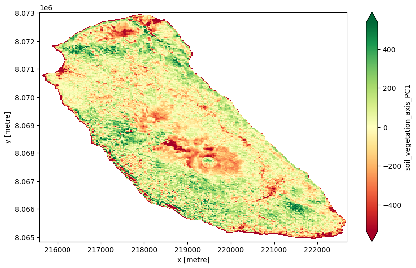
# plot
ax = pc2_da.plot(cmap='RdYlGn', robust=True, figsize=(10, 6))
#ax.set_title('Soil-Vegetation Axis (PC1)', fontsize=14)
plt.show()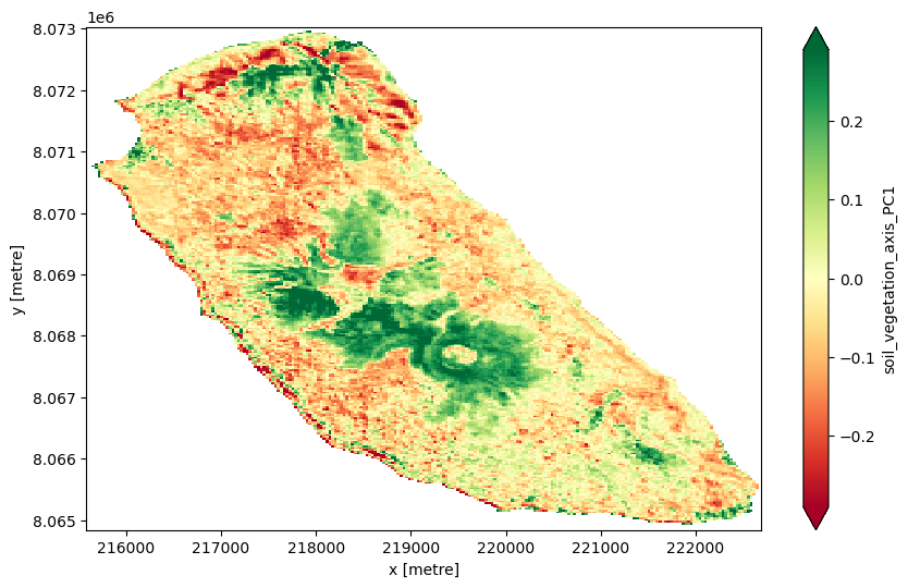
Principal Component 2 (PC2) captures the second largest independent source of variance, orthogonal to PC1. PC2 might represent more subtle or different contrasts in the data, such as:
Variations related to disturbance vs. regrowth (NBR might load more here),
Differences in vegetation structure or type, or
Soil texture or moisture contrasts not fully captured by PC1.
PC2 often helps highlight secondary gradients like areas recovering from disturbance or with different vegetation-soil mixtures.
Let’s check the component loadings:
bands_indices = ['ndmi', 'bsi', 'ndvi', 'msavi2', 'nbr']
loadings_df = pd.DataFrame(pca.components_, columns=bands_indices, index=['PC1', 'PC2'])
print(loadings_df)
ndmi bsi ndvi msavi2 nbr
PC1 0.000247 -0.000270 0.000309 1.000000 0.000247
PC2 -0.508097 0.544503 -0.432654 0.000531 -0.508098
Each loading is a coefficient that tells you how strongly each original variable (index) contributes to a principal component (PC). Loadings can be positive or negative, indicating the direction of the relationship. The magnitude (absolute value) indicates the strength of influence. PC1 loadings show which indices dominate the largest pattern—usually differentiating healthy, moist, dense vegetation (high NDVI, NDMI, MSAVI2) from bare soil or degraded land (high BSI). PC2 loadings capture the next most important pattern, independent of PC1, often related to disturbance, soil texture, or other subtle contrasts.
PC1 shows:
Dominated almost entirely by msavi2 (loading = 1.0)
Other indices have near-zero loadings, so PC1 essentially represents MSAVI2 alone.
Since MSAVI2 is a soil-adjusted vegetation index, PC1 here captures vegetation health adjusted for soil brightness, ignoring other indices.
PC2 shows:
Strong positive loading on bsi (0.54)
Strong negative loadings on ndmi (-0.51), ndvi (-0.43), and nbr (-0.51)
This suggests PC2 contrasts bare soil presence (BSI) with moisture (NDMI), vegetation greenness (NDVI), and disturbance/burn ratio (NBR).
So PC2 likely captures a bare soil vs vegetated/moist/disturbed gradient:
High PC2 values mean more bare soil (high BSI)
Low PC2 values mean more healthy, moist vegetation or recently disturbed areas
PC1 is almost purely MSAVI2, a refined vegetation index accounting for soil brightness. It’s oour main soil-adjusted vegetation axis.
PC2 contrasts bare soil (BSI) with vegetation moisture, greenness, and disturbance — a secondary axis separating exposed soil from vegetated or disturbed areas.
Why is this the case?
Our indices may have very different scales or variance; MSAVI2 dominates variance captured by PC1.
Other indices mainly separate out on PC2, showing a distinct “bare soil vs healthy/disturbed vegetation” gradient.
Takeaways:
Use PC1 as a strong indicator of vegetation health adjusted for soil.
Use PC2 to detect areas with bare soil exposure vs vegetated or disturbed zones.
Can use normalization such as Z-score normalization prior to PCA to account for the different index scales.
Creating a soil health score
We will created a score based on weighted inputs.
The weights
0.45 * ndmi_n → 45% weight to moisture
Soil moisture is a key driver of nutrient cycling and erosion prevention. Given nearly equal weight with NDVI because water availability is just as important as > vegetation cover.
0.45 * ndvi_n → 45% weight to vegetation greenness
Healthy vegetation cover prevents erosion, supports soil organisms, and maintains structure.
0.10 * (1 - bsi_n) → 10% weight to low bare soil exposure
(1 - bsi_n) flips the bare soil index so that less bare soil = higher score. Low bare soil reduces erosion risk and nutrient loss. Smaller weight here because bare soil impact is already partially captured by NDVI and NDMI.
Score range:
0 → low soil health (relatively dry, sparse vegetation, high bare soil).
1 → high soil health (more moisture, greener vegetation, low bare soil exposure).
def calculate_soil_health_score(
    ndmi: xr.DataArray,
    ndvi: xr.DataArray,
    bsi: xr.DataArray,
    weight_ndmi: float = 0.45,
    weight_ndvi: float = 0.45,
    weight_bsi: float = 0.10
) -> xr.DataArray:
    """
    Calculate a soil health score from NDMI, NDVI, and BSI DataArrays.

    The score is a weighted combination of:
    - NDMI (Normalized Difference Moisture Index)
    - NDVI (Normalized Difference Vegetation Index)
    - BSI (Bare Soil Index), inverted so higher vegetation cover improves score

    All indices are automatically normalized to 0–1 range before weighting,
    ignoring NaNs in the normalization calculations.

    Parameters
    ----------
    ndmi : xr.DataArray
        Raw NDMI values.
    ndvi : xr.DataArray
        Raw NDVI values.
    bsi : xr.DataArray
        Raw BSI values.
    weight_ndmi : float, optional
        Weight for NDMI in the score (default 0.45).
    weight_ndvi : float, optional
        Weight for NDVI in the score (default 0.45).
    weight_bsi : float, optional
        Weight for inverted BSI in the score (default 0.10).

    Returns
    -------
    xr.DataArray
        Soil health score scaled between 0 and 1, with NaNs preserved.
    """

    def normalize(da: xr.DataArray) -> xr.DataArray:
        """Normalize a DataArray to the 0–1 range ignoring NaNs."""
        da_min = da.min(skipna=True)
        da_max = da.max(skipna=True)
        return (da - da_min) / (da_max - da_min)

    # Normalize each index (NaNs preserved)
    ndmi_n = normalize(ndmi)
    ndvi_n = normalize(ndvi)
    bsi_n = normalize(bsi)

    # Compute weighted soil health score
    soil_health_score = (
        weight_ndmi * ndmi_n +
        weight_ndvi * ndvi_n +
        weight_bsi * (1 - bsi_n)  # invert BSI so higher vegetation improves score
    )

    # Normalize final score ignoring NaNs
    return normalize(soil_health_score)
score_da = calculate_soil_health_score(s2_data_composite_masked['ndmi'],
s2_data_composite_masked['ndvi'],
s2_data_composite_masked['bsi'])
score_da.plot()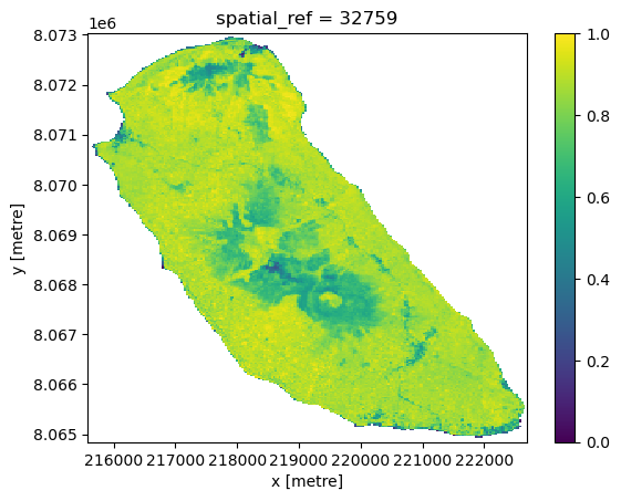
s2_data_composite_masked[["red", "green", "blue"]].to_array("band").plot.imshow(rgb="band", robust=True, size=5, aspect=1)Extra: Add a DEM
Load a DEM to understand elevation’s interplay with soil conditions. Some primary derivatives of a DEM that would be useful here is slope and aspect.
# Connect to Microsoft Planetary Computer STAC
stac_client = Client.open("https://planetarycomputer.microsoft.com/api/stac/v1")

# Search NASA DEM
search = stac_client.search(
    collections=["nasadem"],
    bbox=selected.bounds,
    max_items=1
)

dem_item = planetary_computer.sign(search.item_collection()[0])
dem = odc.stac.load(
items=[dem_item],
crs="EPSG:32759", #4326", # Match with other layers
bbox=selected.bounds, # Same bounding box as the composite
)# Check output ranges
vals = dem["elevation"].isel(valid_time=0).values
vals_clean = vals[np.isfinite(vals)]
print("Unique:", np.unique(vals_clean))
print("Min:", vals_clean.min())
print("Max:", vals_clean.max())s2_data_composite = s2_data_composite.assign(elevation=dem["elevation"])